
COMPLEMENTARITY OF FEATURE POINT DETECTORS
Guillaume Gales, Alain Crouzil
Institut de Recherche en Informatique de Toulouse, Univerist
´
e P. Sabatier
118 rte de Narbonne, 31062 Toulouse cedex 9, France
Sylvie Chambon
Laboratoire Central des Ponts et Chauss
´
ees, rte de Pornic, BP 4129, 44314 Bouguenais cedex, France
Keywords:
Feature points, Complementarity, Repeatability, Spatial distribution.
Abstract:
The goal of this paper is to provide a study on complementarity of feature point detectors. Many studies
have been proposed on these detectors but none deals with complementarity in details. We introduce an
evaluation of eleven well-known detectors based on new criteria used to characterize complementarity. The
complementarity is computed with spatial distribution and contribution measures as well as repeatability and
distribution gains of the association of two detectors.
1 INTRODUCTION
Many applications in computer vision rely on some
characteristic points called feature points (or point of
interest). Their detectors are designed to select the
most distinctive points in an image so they are easy to
match without ambiguities. We asked ourselves the
following question: if different feature point detectors
select the most distinctive points in an image, do they
return the same points ? In other words, we propose
to study the complementary of several feature point
detectors. Previous evaluations studied detection cri-
teria such as repeatability or information content and
matching criteria such as recall and precision rates.
We propose to study the complementarity of feature
point detectors based on new criteria: spatial distri-
bution and complementarity measures. The idea is to
find out which are the most complementary detectors
in order to combine them when needed. Initially, this
evaluation is proposed on small-baseline stereo image
pairs since feature points may be used for instance
in application such as stereo matching (Lhuillier and
Quan, 2002) or fundamental matrix estimation (Hart-
ley and Zisserman, 2004).
First, previous work on feature point detectors is
described. Second, the new criteria to measure com-
plementarity are introduced. Finally, the results of our
experimentations are discussed before the conclusion.
2 PREVIOUS WORK
2.1 Feature Point Detection
Feature points are distinctive points within an image.
Therefore, they are used in many applications such
as tracking, indexation or stereo matching. There are
different families of detectors: contour based, inten-
sity based, parametric model based methods (Schmid
et al., 2000). We focus on intensity based methods
since they are widely used. They are based on the fol-
lowing steps: (i) computation for each pixel of a re-
sponse value based on local grey level variations ; (ii)
non maxima suppression ; (iii) post processing (edge
response elimination, subset selection, subpixel local-
isation). In this section we describe briefly the first
step for the well known detectors: Moravec, Harris,
Kitchen-Rosenfeld, Beaudet, SUSAN, FAST, SIFT,
SURF, Harris-Laplace, Hessian-Laplace and Kadir.
Fixed Scale Detectors. The response is com-
puted using a fixed window size.
Moravec (MO). The response is based on an
auto-correlation measure based on four direc-
tions (Moravec, 1977).
Harris (HA). The response is based on a generali-
sation of the auto-correlation measure on every shift
334
Gales G., Crouzil A. and Chambon S. (2010).
COMPLEMENTARITY OF FEATURE POINT DETECTORS.
In Proceedings of the International Conference on Computer Vision Theory and Applications, pages 334-339
DOI: 10.5220/0002831703340339
Copyright
c
SciTePress

directions. It defines an auto correlation matrix, then
the response is obtained from this matrix. Several
variants were given (Harris and Stephens, 1988; No-
ble, 1988; Shi and Tomasi, 1994).
Kitchen-Rosenfeld (KR). The response is based on
the curvature of the grey level gradients (Kitchen and
Rosenfeld, 1982).
Beaudet (BE). The response is based on the de-
terminant of the Hessian matrix (second deriva-
tives) (Beaudet, 1978).
SUSAN (SU). The response is based on the area in
the neighbourhood of the same intensity as the current
pixel (Smith and Brady, 1997).
FAST (FA). The response is based on the config-
uration of the grey levels on a circle centred on the
current pixel (Rosten and Drummond, 2006).
Multi Scale Detectors. The response is com-
puted using different window sizes (or image resolu-
tions).
SIFT (SI). The response is based on the grey level
Laplacian computed using a difference of Gaus-
sian (Lowe, 1999).
Harris-Laplace, Hessian-Laplace (HAL, HEL).
The response is based on Harris or the Hessian matrix
but the detected feature points must also be maxima
in the scale space of the Laplacian (Mikolajczyk and
Schmid, 2004).
SURF (SR). The response is based on the deter-
minant of the Hessian matrix. The detected feature
points must also be maxima in the scale space of the
determinant of the Hessian (Bay et al., 2006).
Kadir (KA). The response is based on the grey
level histogram entropy of the neighbours of the cur-
rent pixel (Kadir et al., 2004).
2.2 Previous Evaluations
Repeatability. When two images of a same scene
taken under different conditions are submitted to a
feature point detector, it is desirable that the returned
points are repeated: the two projections of a scene
point are detected in the two images. In other words, a
feature point in an image is repeated if its correspon-
dent in the other image is also detected as a feature
point. The repeatability rate of a detector is the per-
centage of repeated points from an image to another.
If this rate is high when a transformation between the
two images is large (rotation, scale change, perspec-
tive change, light change), this detector is robust to
that transformation (Schmid et al., 2000; Mikolajczyk
and Schmid, 2004; Gil et al., 2009).
Information Content. This value represents how
much the feature points of an image are distinct to
each other. The more distinctive the feature points
are, the less ambiguous they are to match. A descrip-
tor is computed for each feature point and the Ma-
hanalobis distance is used to normalize each compo-
nent (Schmid et al., 2000).
Complementarity. The complementarity is mea-
sured in (Mikolajczyk et al., 2005) in an object recog-
nition context. A clustering algorithm is applied to
the feature points, then the number of points from
each detector is computed for each class. Ideally, each
class must contain points from the same detector only.
3 PROPOSED EVALUATION
We propose to extend and modify the previous criteria
with the following ones:
• Spatial Distribution – distribution of feature
points is measured in depth discontinuity areas
and computed region wise ;
• Complementarity – complementarity of two de-
tectors is measured in three ways: contribution
measure ; repeatability gain and distribution gain.
The repeatability is taken into account by the com-
plementarity measures, therefore, we propose to com-
pute it using the definition below.
3.1 Repeatability
Let p
I
i, j
be the pixel at the i
th
row and j
th
column in
the image I. Let d
I
1
i, j
be the disparity vector such as
p
I
2
i
0
, j
0
= p
I
1
i, j
+ d
I
1
i, j
where p
I
2
i
0
, j
0
is the pixel in the right
image which is the projection of the same scene entity
as p
I
1
i, j
. Let ε be a tolerance margin in pixels. We use
the following definitions:
• repeated point – a feature point p
I
1
i, j
in the im-
age I
1
is repeated if a feature point p
I
2
i
0
, j
0
has
been detected in the image I
2
within a distance
lower than ε from its theoretical correspondent,
i.e. ||(p
I
1
i, j
+ d
I
1
i, j
) − p
I
2
i
0
, j
0
|| < ε.
COMPLEMENTARITY OF FEATURE POINT DETECTORS
335

• repeatability rate – the repeatability rate for a de-
tector D and an image pair (I
1
, I
2
) is given by:
rep(I
1
, I
2
) =
rep
D
(I
1
→ I
2
) + rep
D
(I
2
→ I
1
)
2
(1)
with
rep
D
(A → B) =
# feature pts. of A repeated in B
# feature points in A
(2)
3.2 Spatial Distribution
Distribution in Depth Discontinuity Areas. Depth
discontinuity areas are located near the boundaries be-
tween homogeneous depth regions. They result in
grey level variations. However, the grey level of the
background may be locally different for two corre-
spondents which makes such pixels harder to match
than pixels in other areas. Feature point detectors tend
to select points in areas where high grey level varia-
tions occur and therefore may return points in depth
discontinuity areas. Thus, we compute the following
measure:
DA =
# feature points in depth discontinuity areas
# feature points
(3)
Region Wise Distribution. The regions are ex-
tracted using a color segmentation algorithm. The
idea is based on the hypothesis that pixels with more
or less the same color belong to the same object part
(and therefore have more or less the same disparity
value). For a detector D, the region wise distribution
score is:
RD
D,S
=
# regions holding at least one feature point
# regions
(4)
where S is a segmentation map. A low ratio reveals
a lack of feature points or a bad distribution over the
different regions of the image.
3.3 Complementarity
Contribution Measure. Let P
D
1
be the set of the
feature points returned by a detector D
1
and P
D2
the
set of the feature point returned by a detector D
2
. The
contribution of D
2
over D
1
is given by:
contribution
D
2
|D
1
=
card
{
P
D
2
}
− card
{
P
D
1
∩ P
D
2
}
card
{
P
D
1
}
(5)
where the intersection P
D
1
∩ P
D
2
is computed consid-
ering two points p
I
i, j
and p
I
i
0
, j
0
of an image I as the
50 100 150 200 250 300 350 400 450
50
100
150
200
250
300
350
50 100 150 200 250 300 350 400 450
50
100
150
200
250
300
350
P
HA
P
BE
− (P
HA
∩ P
BE
)
Figure 1: This figure shows on the left all the feature points
returned by HA and on the right the contribution of BE, i.e.
the feature points returned by BE which are different from
the ones already returned by HA (ε = 3). It also shows the
segmentation map (each color represents one region).
same point when ||p
I
i, j
− p
I
i
0
, j
0
|| < ε. The higher this
value is with a high ε, the larger the differences are
between the two sets P
D
1
and P
D
2
. This measure is
illustrated by figure 1.
This contribution measure is not symmetric since
the cardinalities of each detector are different, there-
fore in order to get an objective idea of the comple-
mentarity of the union of two detectors (D
1
, D
2
), we
compute:
contribution(D
1
, D
2
) = contribution(D
2
, D
1
)
= min(contribution
D
2
|D
1
, contribution
D
1
|D
2
)
(6)
Repeatability Gain. The repeatability is computed
independently for the detectors D
1
and D
2
. It is then
computed with D
1
&D
2
which represents the union
P
D
1
∪ P
D
2
. The gain of repeatability is given by:
gain
rep
D
1
&D
2
= rep
D
1
&D
2
− max
rep
D
1
, rep
D
2
(7)
Distribution Gain. The spatial distribution is com-
puted independently for the detectors D
1
and D
2
. It
is then computed with D
1
&D
2
which represents the
union P
D
1
∪ P
D
2
. The gain of distribution is given by:
gain
RD
D
1
&D
2
,S
=RD
D
1
&D
2
,S
− max(RD
D
1
,S
, RD
D
2
,S
)
(8)
where S is a segmentation map.
4 DATA SET
4.1 Stereo Pairs
Stereo pairs from the Middlebury data set
1
are used
for this experimentation
2
. They present issues such as
1
vision.middlebury.edu/stereo/data/
2
We use the pairs named aloe, art, bowling1, cloth1,
cloth4, cones, dolls, midd2, moebius, plastic and teddy.
VISAPP 2010 - International Conference on Computer Vision Theory and Applications
336
occlusions and depth discontinuities. They are epipo-
lar rectified and the ground truth is known. However,
deformations between two images is not as important
as it could occur in applications such as indexation.
4.2 Implementation Details
The programs provided by the detector authors is used
when available: HAL
3
, HEL
4
, SU
5
, FA
6
, SI
7
, SR
8
and KA
9
. Our own implementation is used for the
other detectors. For each detector, the following pa-
rameters can have an influence on the result:
• Response Window Size (for fixed scale detectors)
– the smaller this size is, the more the detector is
able to select small structures but the greater the
noise sensitivity is. On the other hand, the greater
this size is, the larger the smoothing effect is and
the greater localization errors are.
• Non Maxima Suppression Window Size – the
smaller this size is, the larger the number of de-
tected feature points is but these feature points
may be close to each other.
• Response Threshold – a threshold on the response
value is often used in order to get rid of false re-
sponses. The higher this value is, the smaller the
number of feature points is.
It would be interesting to study the influence of each
parameter on the result but this exhaustive evaluation
is difficult to analyse. Moreover, for the detectors im-
plemented by their authors, we do not always have the
possibility to change all the settings. A normalization
would also be necessary on all the different values in
order to make them comparable. Facing this issue, we
decided to fix these parameters once for all for each
detector. For the detectors we implemented, we used
parameter values that give good results with our ex-
perimentations. For the the other detectors, we used
the default values given by their authors.
5 RESULTS
5.1 Repeatability
The repeatability rep
D
of a detector D is given by
computing the mean value of the repeatability rates
3
robots.ox.ac.uk/˜vgg/research/affine/
4
robots.ox.ac.uk/˜vgg/research/affine/
5
users.fmrib.ox.ac.uk/˜steve/susan/index.html
6
svr-www.eng.cam.ac.uk/˜er258/work/fast.html
7
cs.ubc.ca/spider/lowe/keypoints/siftDemoV4.zip
8
vision.ee.ethz.ch/˜surf/
9
robots.ox.ac.uk/˜timork/salscale.html
0 1 2 3
0
10
20
30
40
50
60
¡
Repeatability (%)
BE
FA
HAL
HA
HEL
KA
KR
MO
SI
SR
SU
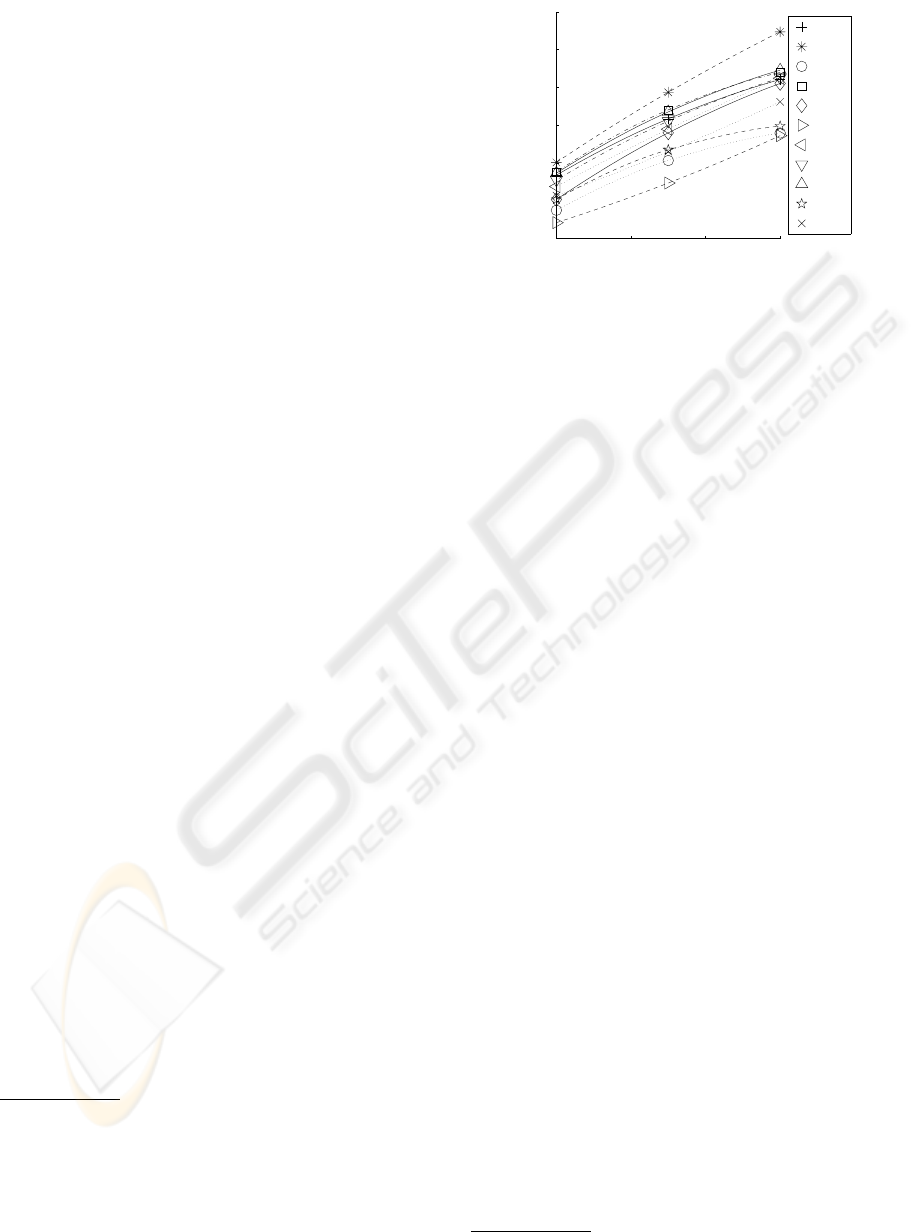
Figure 2: Repeatability scores rep
D
for the tested detectors.
All the feature points are taken into account, therefore fea-
ture points in occluded areas decrease the score. The nota-
tions are defined in § 2.1.
found over the data set. The repeatability is mea-
sured by taking ε ∈
{
0, 1.5, 3
}
. The results for re-
peatability are shown in figure 2. The detectors with
the best repeatability are HA, FA and SI. For ε = 0
the repeatabilities are very low. Therefore, a “fea-
ture points to feature points” matching strategy is not
advisable when high precision is required. We rec-
ommend a “feature points to neighbours of feature
points” matching strategy to settle this issue.
5.2 Spatial Distribution
The results for the depth discontinuity distribution are
shown in table 1. The depth discontinuity areas are
computed using the provided ground truth disparity
maps, see § 4.1. The results for the region wise dis-
tribution are shown in table 1. The EDISON
10
pro-
gram is used to compute two segmentation maps: (i)
an “under” segmentation S1 giving about 100 regions
for each image ; (ii) a “medium” segmentation S2 giv-
ing about 500 regions for each image (see figure 1).
The most significant criteria, where the biggest
differences are obtained, are RD
D,S2
and Card. HAL
detector returns very few points and consequently
gives also the worst RD
D,S2
. On the other hand,
HA detector seems to obtain the best compromise
between cardinality, DA and RD
D,S2
. According to
these results, the best compromises is obtained by the
detectors HA, FA and SI.
5.3 Complementarity
Contribution Measure. This measure is computed
over all the feature points and over the repeated points
with ε = 3 (we consider this value as the minimum
10
caip.rutgers.edu/riul/research/code/EDISON/
COMPLEMENTARITY OF FEATURE POINT DETECTORS
337

Table 1: Mean cardinalities (Card.), mean of the distribu-
tion measures in depth discontinuity (DA), and mean of the
region based distribution measure (RD) with segmentation
S1 ans S2. For each column the best result is shown in bold.
D Card. DA% RD
D,S1
% RD
D,S2
%
BE 967 28 100 78
FA 2243 27 100 83
HAL 293 35 94 30
HA 989 25 99 86
HEL 1252 32 100 73
KA 638 29 99 61
KR 1153 31 100 81
MO 845 27 97 62
SI 1662 29 99 82
SR 303 31 99 49
SU 922 29 100 74
distance between two different points) in one hand
and ε = 12 (large enough value to see which detec-
tors return complementary feature points away from
each other) on the other hand. The results are shown
in table 2 (the measures are computed over all the fea-
tures points) and in table 3 (the measures are com-
puted over the repeated feature points). According to
these results, the most complementary detectors are
KA+SU, KA+MO and KR+HEL. By reading these
tables, we can see for instance that by taking the union
HA+SI, we add in the worst case 67% of new repeated
feature points within a distance of ε = 3 pixels of each
other and 2% of new repeated feature points within a
distance of ε = 12 (i.e. at least 12 pixels farther than
the already computed feature points).
Repeatability Gain. The results are shown in ta-
ble 4. They show which detectors are the most com-
plementary in terms of repeatability. First, it shows
the good complementarity of the following detectors
KR+HEL, HEL+SU and KR+SI. Second, it shows
which detector to use in combination to another in or-
der to improve the repeatability. The best repeatabil-
ity was given by FA, see § 5.1. Therefore, adding the
feature points from the detector HEL can improve by
2.12% the repeatability of FA.
Distribution Gain. The segmentation S2 is used
in our experimentation, see § 5.2. The results are
shown in table 5. They show which detectors are
the most complementary in terms of region based
distribution. First, it shows the good complementar-
ity of the following detectors KA+MO, KA+SU and
KA+SR. Second, it shows which detector to use in
combination to another in order to improve the spatial
distribution. The best region based distribution was
given by HA, see § 5.2. By reading table 5, we can
see that adding the feature points from the detector BE
can improve the distribution by 6.14% which gives a
Table 2: Contribution measures taking into account all the
feature points. For each couple of detectors D
1
&D
2
, we
show contribution
D
2
|D
1
. ε = 3 on the first row and ε = 12
on the second row. To find out which detector is the most
complementary with HA and ε = 3, for instance, look at the
HA row and column (here in blue). It shows that it is HEL.
For each detector and each ε value, the best result appears
in bold.
BE FA HAL HA HEL KA KR MO SI SR
FA
17 0
4 0
HAL
20 9 0
2 1 0
HA
55 28 15 0
2 2 0 0
HEL
58 56 9 67 0
10 10 0 6 0
KA
56 28 40 56 49 0
19 12 9 9 15 0
KR
58 18 23 62 73 58 0
8 2 1 1 9 20 0
MO
39 4 39 42 53 85 27 0
2 0 8 10 5 27 1 0
SI
37 28 16 56 58 45 51 31 0
7 3 1 2 10 20 5 2 0
SR
23 13 70 25 3 38 26 46 10 0
3 1 8 1 0 9 2 12 1 0
SU
42 6 36 42 55 92 33 45 32 39
3 0 3 1 6 30 2 3 3 5
Table 3: Contribution measures taking into account the re-
peated feature points (see table 2 for notations).
BE FA HAL HA HEL KA KR MO SI SR
FA
18 0
6 0
HAL
19 7 0
2 1 0
HA
52 30 12 0
3 3 0 0
HEL
61 51 8 75 0
13 12 1 6 0
KA
34 19 71 33 32 0
17 14 11 7 16 0
KR
68 17 22 60 72 42 0
9 2 1 1 11 22 0
MO
46 5 36 44 55 82 35 0
2 0 10 0 6 31 1 0
SI
42 27 15 67 63 29 53 34 0
8 4 1 2 13 21 6 2 0
SR
21 9 85 20 3 64 24 42 8 0
3 1 12 1 0 11 2 13 1 0
SU
42 5 43 36 47 85 35 62 29 41
3 1 3 1 7 37 2 3 3 5
score of 86+6.14=92.14% for the union HA+BE.
Analysis. These results can be read in two ways: (i)
for each detector they give which detector is the most
complementary in terms of contribution, repeatability
and spatial distribution ; (ii) they give the most com-
plementary detectors between them. The best com-
promises between repeatability and distribution are
given by: Harris, FAST and SIFT. Table 6 summa-
VISAPP 2010 - International Conference on Computer Vision Theory and Applications
338

Table 4: Repeatability gain. For each couple of detectors
D
1
&D
2
, we show gain
rep
D
1
&D
2
(ε = 3). To determine which
detector is the most complementary in terms of repeatability
with HA, for instance, look at the HA row and column (here
in blue), it shows that it is HEL. For each detector, the best
result appears in bold.
BE FA HAL HA HEL KA KR MO SI SR
FA 1.55 0
HAL 0.75 -0.36 0
HA 3.77 0.32 -0.36 0
HEL 4.48 2.12 0.36 4.20 0
KA -0.17 -1.69 -0.39 -0.38 2.03 0
KR 4.71 0.22 0.90 3.88 5.75 1.81 0
MO 3.78 -0.69-0.62 3.11 4.47 -1.34 2.83 0
SI 3.57 1.19 0.76 3.40 2.37 0.82 4.98 3.00 0
SR 1.01 0.38 0.09 0.66 -2.06 1.48 1.70 0.82 -0.19 0
SU 3.53 -1.21 1.65 2.24 5.00 2.60 3.50 2.23 2.46 2.63
Table 5: Distribution gain. For each couple of detectors
D
1
&D
2
, we show gain
RD
D
1
&D
2
,S2
(ε = 3) (see 4 for an exam-
ple of how to read the table).
BE FA HAL HA HEL KA KR MO SI SR
FA 3.96 0
HAL 2.23 1.30 0
HA 6.14 5.11 1.19 0
HEL 8.13 7.80 1.30 6.09 0
KA 8.53 6.85 7.09 5.54 9.27 0
KR 6.47 4.23 3.28 5.86 7.98 6.08 0
MO 3.82 0.02 6.46 3.26 8.62 12.07 2.30 0
SI 5.32 4.96 1.52 5.95 5.39 6.88 6.12 2.92 0
SR 4.15 3.79 4.89 3.63 0.51 11.58 5.30 10.38 1.71 0
SU 6.16 0.10 3.30 4.18 9.72 10.17 3.20 3.27 4.45 7.12
rizes the most complementary detectors to the detec-
tors in terms of contribution, repeatability and region-
wise distribution. The most complementary detectors
between them are Kadir and SUSAN, Kitchen and
Rosenfeld and Hessian-Laplace, Moravec and Kadir
i.e. they return the most distinct sets of feature points.
Table 6: This table summarizes the most complementary
detectors to Harris, FAST and SIFT in terms of contribution
(Cont.) (ε = 3) (results are similar whether all the feature
points or only the repeated points are taken into account),
repeatability (R) and region based distribution (RD
S2
).
D Cont. R RD
D
1
&D
2
,S2
HA HEL HEL BE
FA HEL HEL HEL
SI HEL KR KA
6 CONCLUSIONS
We proposed an evaluation and a comparison of
eleven well-known feature point detectors based on
new criteria used to characterize spatial distribution
and complementarity. This study aims to be helpful
for any applications that need feature points well dis-
tributed in the image. It also helps to select the most
complementary detectors in terms of region based dis-
tribution. This work will be extended on larger trans-
formations between the images.
REFERENCES
Bay, H., Ess, A., Tuytelaars, T., and Gool, L. V. (2006).
SURF: Speeded up robust features. CVIU, pages 346–
359.
Beaudet, P. R. (1978). Rotationally invariant image opera-
tors. In ICPR, pages 579–583, Kyoto, Japan.
Gil, A., Martinez, O., Ballesta, M., and Reinoso, O. (2009).
A comparative evaluation of interest point detectors
and local descriptors for visual SLAM. MVA.
Harris, C. and Stephens, M. (1988). A combined corner
and edge detector. In Alvey Vision Conference, pages
147–151, Manchester, United-Kingdom.
Hartley, R. I. and Zisserman, A. (2004). Multiple View Ge-
ometry in Computer Vision. Cambridge University
Press, ISBN: 0521540518, second edition.
Kadir, T., Zisserman, A., and Brady, M. (2004). An affine
invariant salient region detector. In ECCV, pages 404–
416, Prague, Czech Republic.
Kitchen, L. and Rosenfeld, A. (1982). Gray level corner
detection. PRL, 1(2):95–102.
Lhuillier, M. and Quan, L. (2002). Match propagation
for image-based modeling and rendering. PAMI,
24(8):1140–1146.
Lowe, D. G. (1999). Object recognition from local scale-
invariant features. In ICCV, volume 2, pages 1150–
1157, Kerkyra, Greece.
Mikolajczyk, K., Leibe, B., and Schiele, B. (2005). Local
features for object classe recognition. In ICCV, vol-
ume 2, pages 1792–1799, Beijing, China.
Mikolajczyk, K. and Schmid, C. (2004). Scale & affine
invariant interest point detectors. IJCV, 60(1):63–86.
Moravec, H. P. (1977). Toward automatic visual obstacle
avoidance. In IJCAI, volume 2, pages 584–584, Mas-
sachusetts, USA.
Noble, J. A. (1988). Finding corners. IVC, 6(2):121–128.
Rosten, E. and Drummond, T. (2006). Machine learning
for high-speed corner detection. In ECCV, volume 1,
pages 430–443, Graz, Austria.
Schmid, C., Mohr, R., and Bauckhage, C. (2000). Evalua-
tion of interest point detectors. IJCV, 37(2):151–172.
Shi, J. and Tomasi, C. (1994). Good features to track. In
CVPR, pages 593–600, Seattle, USA.
Smith, S. M. and Brady, J. M. (1997). Susan – a new ap-
proach to low level image processing. IJCV, 23(1):45–
78.
COMPLEMENTARITY OF FEATURE POINT DETECTORS
339
