FORMATION CONTROL OF MULTI-ROBOTS VIA SLIDING-MODE

TECHNIQUE

Razvan Solea, Daniela Cernega, Adrian Filipescu and Adriana Serbencu

Control Systems and Industrial Informatics Department, Computer Science Faculty

“Dunarea de Jos” University of Galati, Domneasca 111, 800201, Galati, Romania

Keywords:

Formation control, Sliding-mode control, Skid-steering mobile robot.

Abstract:

This paper addresses the control of a team of nonholonomic mobile robots. Indeed, the most work, in this

domain, have studied extensively classical control for keeping a formation of mobile robots. In this work, the

leader mobile robot is controlled to follow an arbitrary reference path, and the follower mobile robot use the

sliding-mode controller to keep constant relative distance and constant angle to the leader robot. The efﬁciency

and simplicity of this control laws has been proved by simulation on different situations.

1 INTRODUCTION

The multi robots systems is an important robotics re-

search ﬁeld. Such systems are of interest for many

reasons; tasks could be too complex for a simple robot

to accomplish; using several simple robots can be eas-

ier, cheaper and more ﬂexible than a single power-

ful robot (Mazo et al., 2004), (Zavlanos and Pappas,

2008), (Murray, 2007), (Liu et al., 2007), (Klanˇcar

et al., 2009).

Formation control has been one of the important

research topics in multiple robot systems as it is appli-

cable to many areas such as geographical exploration,

rescue operations, surveillance, mine sweeping, and

transportation. Different approaches have been devel-

oped recently, for example, behavior-based control,

LQ control, visual servoing control, Lyapunov-based

control, input and output feedback linearization con-

trol, graph theory, and nonlinear control.

In leader-follower formation control, the most

widely used control technique is feedback lineariza-

tion based on the kinematics model of the system. In

this study, we focus on the problem of leader-follower

robot formation control using a sliding-mode con-

troller.

The referenced robot is called a leader, and the

robot following it called a follower. Thus, there are

many pairs of leaders and followers and complex for-

mations can be achieved by controlling relative posi-

tions of these pairs of robots respectively. This ap-

proach is characterized by simplicity, reliability and

no need for global knowledge and computation.

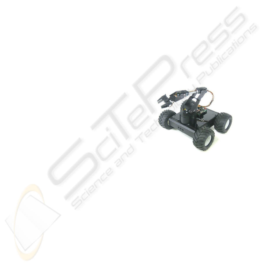
Figure 1: A skid-steered four wheel mobile robot.

In this paper, it will be developped a method based

on the leader-following approach to investigate for-

mation control problem in a group of nonholonomic

mobile robots. For this purpose, we design a new con-

troller based on sliding-mode control to drive a ﬂeet

of mobile robots in a leader-follower conﬁguration.

Sliding Mode Control (SMC) method has been

widely noticed because of its superior robust con-

trol performance for systems with highly uncertainty

(Chwa, 2004), (Yang and Kim, 1999), (Floquet et al.,

2003), (Solea and Nunes, 2007), (Solea and Cernega,

2009).

The rest of this paper is organized as follows. First

formulation of the nonholonomic mobile robot sys-

tem is revealed. Then, the leader-following formation

model method used by the robots is exposed. After

that, the architecture of the siling-mode controller is

described. This paper concludes with some simula-

tion and results.

161

Solea R., Cernega D., Filipescu A. and Serbencu A. (2010).

FORMATION CONTROL OF MULTI-ROBOTS VIA SLIDING-MODE TECHNIQUE.

In Proceedings of the 7th International Conference on Informatics in Control, Automation and Robotics, pages 161-166

DOI: 10.5220/0002899501610166

 SciTePress

2 FORMATION CONTROL

2.1 Formulation of the Nonholonomic

Mobile Robot System

As indicated in Figure 1, the mobile robots are skid-

steering mobile platforms. To develop the kinematic

model for a skid-steering mobile robot (SSMR) that

is assumed to move in a plane (for simplicity) with an

inertial coordinate system, denoted by (X

, Y

), and

a local coordinate system, denoted by (X

, Y

), where

the origin of (X

, Y

) is ﬁxed to the center of mass

(CG) of the SSMR as illustrated in Figure 2. The po-

sition and orientation of the CG, denoted by q(t) ∈ R

is deﬁned as q = [x

]

(i.e., the CG position, x

and y

, and the orientation θ

of the local coordinate

frame with respect to the inertial frame).





˙x

˙y









cos(θ

) −sin(θ

) 0

sin(θ

) cos(θ

) 0

0 0 1













(1)

It is obvious that Eqn. (1) does not impose any

restrictions on the skid-steering mobile robot plane

movement, since it describes free-body kinematics

only. Therefore it is necessary to analyze the relation-

ship between wheel velocities and local velocities.

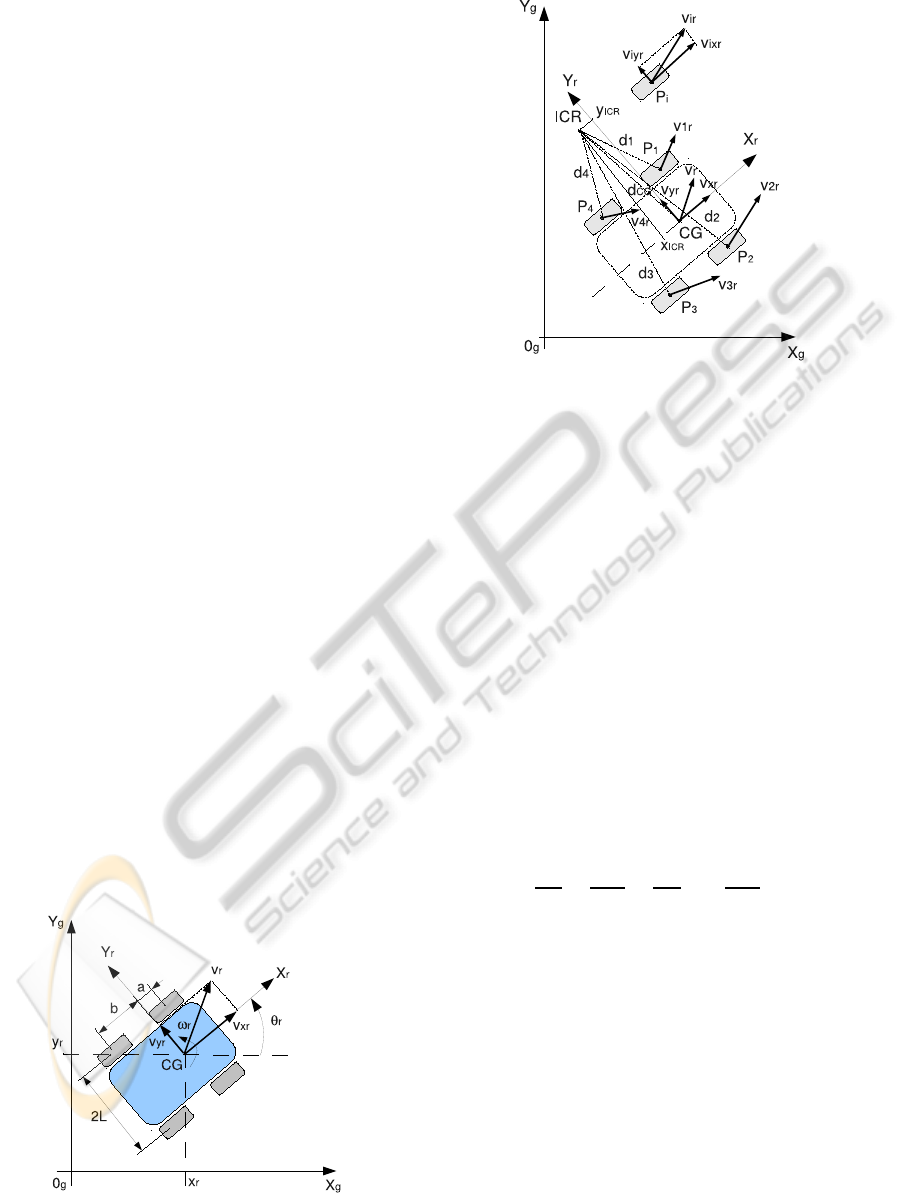
Suppose that the i − th wheel rotates with an an-

gular velocity ω

(t), where i = 1, 2,...,4, which can

be seen as a control input. For simplicity, the thick-

ness of the wheel is neglected and is assumed to be

in contact with the plane at point P

as illustrated in

Figure 3. In contrast to most wheeled vehicles, the lat-

eral velocity of the SMRR, v

iyr

, is generally nonzero.

This property comes from the mechanical structure of

the SSMR that makes lateral skidding necessary if the

vehicle changes its orientation. Therefore the wheels

are tangent to the path only if ω

= 0, i.e., when the

robot moves along a straight line.

Figure 2: Free body diagram.

Figure 3: Wheel velocities.

In this description we consider only a simpliﬁed

case of the SSMR movement for which the longitudi-

nal slip between the wheels and the surface can be ne-

glected. For traditional mobile robots, the wheel rota-

tion is translated into a linear motion along the tangent

of a curve without longitudinal slippage as described

by the following expressions:

ixr

= R

· ω

(2)

where v

ixr

is the longitudinal component of the total

velocity vector v

of the i − th wheel expressed in

the local frame and R

denotes the so-called effective

rolling radius of that wheel.

The vectors d

(t) = [d

(t),d

(t)]

and d

(t) =

CGx

(t),d

CGy

(t)]

∈ R

are expressed in (X

) and

are deﬁned from the instantaneous center of rotation

(ICR) of the vehicle to P

∀i = 1,2,...,4 and d

(t)

from the ICR to the vehicle to CG, respectively, as il-

lustrated in Figure 3. Based on the geometry of Figure

3, the following expressions can be developed:

ixr

ICR

iyr

= −

ICR

= ω

(3)

where it is used the fact that the coordinates of the ICR

expressed in (X

), denoted by x

ICR

(t) and y

ICR

(t) ∈

R, are deﬁned as [x

ICR

]

= [−d

CGx

CGy

]

From Figure 3 it is clear that the coordinates of

vectors d

satisfy the following relationships:

= d

CGy

− L

= d

CGy

+ L

= d

CGx

+ a

= d

CGx

− b

(4)

After combining Eqns. (3) and (4), the follow-

ing relationships between wheel velocities can be ob-

tained:

= v

1xr

= v

4xr

= v

2xr

= v

3xr

= v

1yr

= v

2yr

= v

3yr

= v

4yr

(5)

ICINCO 2010 - 7th International Conference on Informatics in Control, Automation and Robotics

162

where v

and v

denote the longitudinal coordinates

of the left and right wheel velocities, v

and v

are

the lateral coordinates of the velocities of the front

and rear wheels, respectively.

Using (3) - (5) it is possible to obtain the fol-

lowing transformation describing the relationship be-

tween the wheel velocities and the velocity of the

robot:



















1 −L

1 L

0 −x

ICR

+ a

0 −x

ICR

− b











(6)

Notice that ω

and ω

which denote angular ve-

locities of left and right wheels, respectively, can be

regarded as control inputs at kinematic level and can

be used to control longitudinal and angular velocity

according to the following relationships:

= R·

+ ω

, ω

= R·

− ω

2· L

(7)

while R is so called effective radius of wheels and 2·L

is a spacing wheel track depicted in Figure 2.

It is interesting to see that the analysed kinematic

model of the SSMR is quite similar to the kinematics

of the two-wheel mobile robot.

From the last equations it is clear that, theoreti-

cally, the pair of velocities ω

and ω

can be treated

as a control kinematic input signal as well as veloc-

ities v

and ω

. However, the accuracy of the rela-

tions (7) mostly depends on the longitudinal slip and

can be valid only if this phenomenon is not dominant.

In addition, the parameters R and L may be identiﬁed

experimentally to ensure a high validity of the deter-

mination of the angular robot velocity with respect to

the angular velocities of the wheels.

To complete the kinematic model of the SSMR,

the following velocity constraint can be considered:

+ x

ICR

· ω

= 0 (8)

The last equation is not integrable. In conse-

quence, it describes a nonholonomic constraint which

can be rewritten like:



−sin(θ

) cos(θ

) x

ICR







˙x

˙y





= 0 (9)

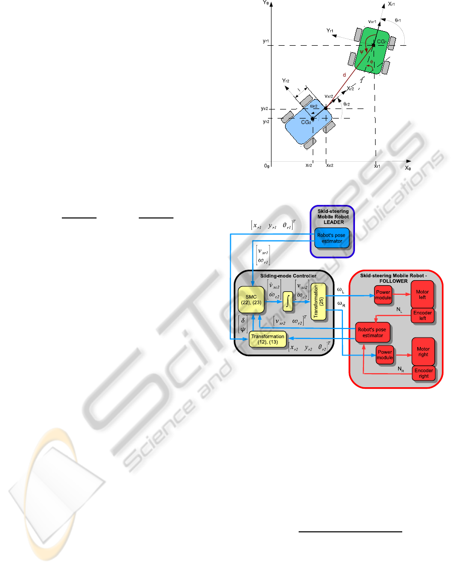
2.2 Leader-follower Formation Models

Figure 4 is a leader-follower control model where the

formation pattern is speciﬁed by the separate distance

d and the relative bearing ψ for two robots r1 and r2.

The desired formation pattern can be deﬁned as the

desired separate distance d

and the relative bearing

Figure 4: Leader-follower approach for SSMR.

Figure 5: Block diagram.

. The follower r2 regulates the formation state er-

rors of the separate distance and the relative bearing

through its speed control signals u

= [v

xr2

,ω

]









−





(10)

The relative distance between the leader and the

follower robot is denoted as d, the separation bearing

angle is ψ, and they are given by:

d =

− x

)

+ (y

− y

)

(11)

ψ = π − [θ

− arctan2(y

− y

− x

)] (12)

where:

= x

+ l · cos(θ

), y

= y

+ l · sin(θ

)

The formation control can be investigatedby mod-

eling the formation state error as follows (Das et al.,

FORMATION CONTROL OF MULTI-ROBOTS VIA SLIDING-MODE TECHNIQUE

163

2002):





= G· u

+ F · u

φ = ω

− ω

(13)

and

G =

−cos(φ+ ψ) −l · sin(φ+ ψ)

sin(φ+ ψ)

−

l · cos(φ + ψ)

F =

cos(ψ) 0

−

sin(ψ)

where φ = θ

− θ

and l is the distance between the

robot position (x

) and the robot hand position

) as shown in Figure 4.

2.3 Sliding-mode Controller Design

In a leader-follower conﬁguration, with the leader’s

position given and once the follower’s relative dis-

tance and angle with respect to the leader are known,

the follower’s position can be determined. To use the

leader-following approach, it is assumed that the an-

gular and linear velocities of the leader are known.

In order to achieve and maintain the desired forma-

tion between the leader and follower, it is only need to

control the follower’s angular and linear velocities to

achieve the relative distance and angle between them

as speciﬁed. Therefore, the leader-following based

mobile robot formation control can be considered as

an extension of the tracking control problem of the

nonholonomic mobile robot.

A practical form of reaching the control law (pro-

posed by Gao and Hung (Gao and Hung, 1993)) is

deﬁned as

˙s

= −p

· |s

· sgn(s

), 0 < α < 1, i = 1,2 (14)

This reaching law increases the reaching speed

when the state is far away from the switching man-

ifold, but reduces the rate when the state is near the

manifold. The result is a fast reaching and low chat-

tering reaching mode.

A new design of sliding surface is proposed, such

that the separation bearing angle, ψ and the orienta-

tion error φ, are internally coupled with each other in

a sliding surface leading to convergence of both vari-

ables. For that purpose the following sliding surfaces

is proposed:

d + γ

d (15)

ψ+ γ

· sgn(

ψ) · | φ| (16)

here γ

, γ

are positive constant parameters and

ψ, φ are deﬁned by (10), (13).

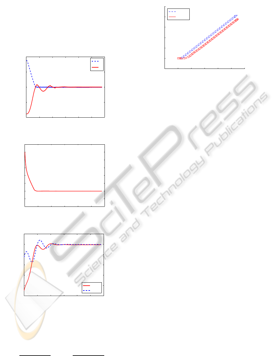
−4 −2 0 2 4 6

−2

Trajectory

x [m]

y[m]

leader

follower

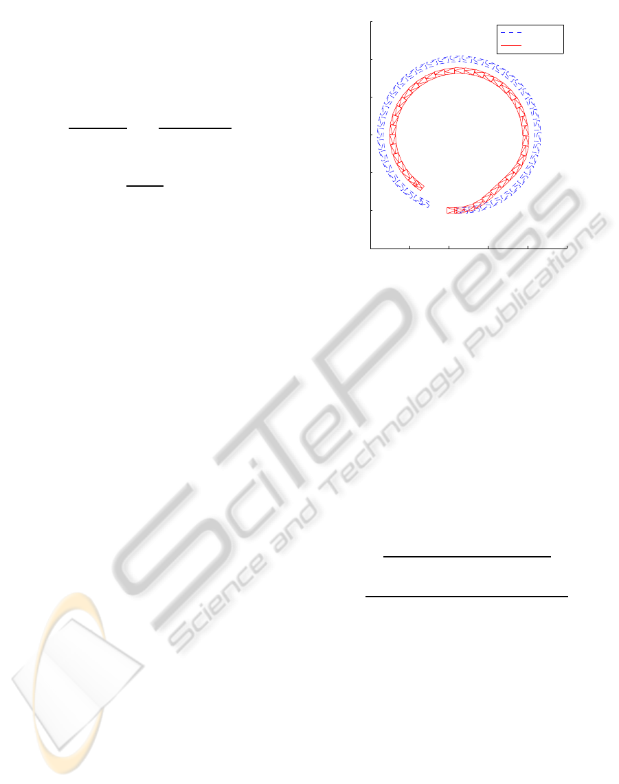
Figure 6: Simulation I - Trajectory of the leader and the

follower.

If s

converges to zero, trivially

d converges to

zero. If s

converges to zero, in steady-state it be-

comes

ψ = −γ

ψ− γ

· sgn(

ψ) · |φ|. Since |φ| is al-

ways bounded, the following relationship between

and

ψ holds:

ψ < 0 ⇒

ψ > 0 and

ψ > 0 ⇒

ψ < 0.

From the time derivative of (15) and (16) and us-

ing the reaching law deﬁned in (14) yields:

˙s

d + γ

d = −p

· |s

· sgn(s

) (17)

˙s

ψ+ γ

· sgn(

ψ) · sgn(

φ) ·

φ =

= −p

· |s

· sgn(s

)

(18)

After some mathematical manipulation, one can

achieve:

˙v

xc2

· |s

· sgn(s

) + γ

d − D

cos(φ+ ψ)

(19)

· |s

· sgn(s

) + γ

psi

ψ) · d − D

l · cos(φ+ ψ)

(20)

where

= l ·

· sin(φ + ψ) − d· (

φ+

ψ) · (

ψ+ ω

)−

− ˙v

xr1

· cos(ψ) − v

xr1

φ· sin(ψ)

= γ

· sgn(

ψ· φ) ·

φ· d − ˙v

xr2

· sin(φ + ψ)+

+ ˙v

rx1

· sin(ψ) − v

xr1

φ· cos(ψ) − (

φ+

ψ) ·

d−

−d ·

−

d · (

ψ+ ω

)

The signum functions in the sliding surface were

replaced by saturation functions, to reduce the chat-

tering phenomenon (Slotine and Li, 1991).

3 SIMULATION RESULTS

In this section, simulation results for the proposed

SMC are presented. The simulation are performed

ICINCO 2010 - 7th International Conference on Informatics in Control, Automation and Robotics

164

in Matlab/Simulink environment to verify behavior of

the controlled system. The parameters of the SSMR

model were chosen to correspond as closely as possi-

ble to the real experimental robot presented in section

1 in the following manner: a = 0.10[m], b = 0.20[m],

L = 0.12[m], R = 0.04[m]. Wheel velocity commands,

0 10 20 30 40 50 60

−0.4

−0.2

0.2

0.4

Sliding surfaces s

and s

time [s]

, s

(a)

0 10 20 30 40 50 60

−0.2

−0.1

0.1

0.2

0.3

0.4

0.5

0.6

Separate distance

time [s]

d tilde [m]

(b)

0 10 20 30 40 50 60

−50

−40

−30

−20

−10

Relative bearing (ψ tilde) and relative orientation (φ)

time [s]

ψ tilde, φ [deg]

ψ tilde

(c)

Figure 7: Simulation I - Sliding surfaces s

and s

, separate

distance (

d), relative bearing (

ψ) and relative orientation

(φ).

xc2

+ L· ω

; ω

xc2

− L· ω

; (21)

are sent to the power modules of the follower mobile

robot, and encoder measures NR and NL are received

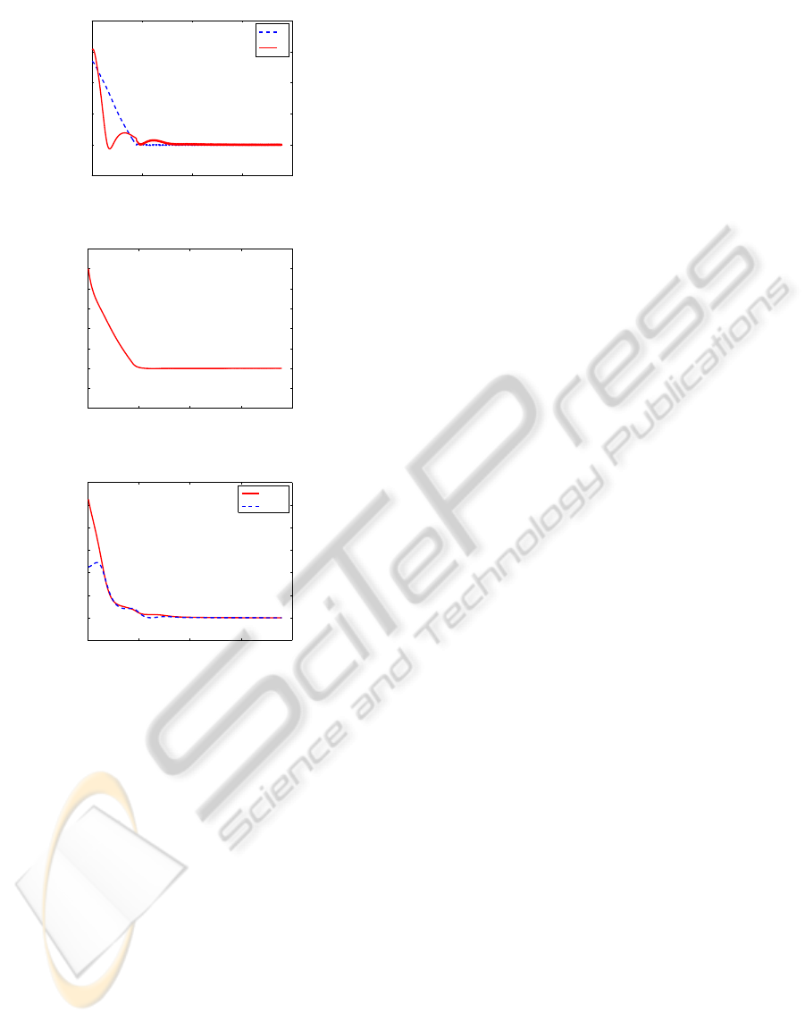
−2 0 2 4 6 8 10

−2

Trajectory

x [m]

y[m]

leader

follower

Figure 8: Simulation II - Trajectory of the leader and the

follower.

in the robots pose estimator for odometric computa-

tions.

Figure 5 shows a block diagram of the proposed

sliding-mode controller.

In order to compute the actuating control input,

equation (6) needs to be integrated and some initial

values v

xc2

(0), ω

(0) to be ﬁxed.

Two simulation experiments were carried out to

evaluate the performance of the sliding mode con-

troller presented in Section 2.3. The ﬁrst simula-

tion refers to the case of circular trajectory (v

xr1

0.4[m/s] and ω

= 0.1[rad/s]). The initial condi-

tions of the leader and the follower are, x

(0) =

0.5, y

(0) = 0, θ

(0) = 0, x

(0) = 0, y

(0) = 0,

(0) = 0, d

= 1.0[m], ψ

= 135[deg].

In the second simulation the leader robot execute a

linear trajectory but with a non-zero initial orietation

(θ

= 45[deg]). The initial conditions of the leader

and the follower in this second case are, x

(0) = 0.5,

(0) = 0, θ

(0) = pi/4, x

(0) = 0, y

(0) = 0,

(0) = 0, d

= 1.0[m], ψ

= −120[deg].

Figure 6 shows the trajectory of the leader and the

follower for the ﬁrst simulation case. In order to have

a temporal reference in the ﬁgure the robots are drawn

each second: the blue car represent the leader and the

red car represent the follower.

In Figure 7.a the sliding surfaces s

and s

asymp-

totically converge to zero. Finally, Figures 7.b and c

show the time histories of

ψ and φ.

The results of the second case called Simulation

II are given in Figures 8 - 9. Figure 8 shows the tra-

jectory of the leader and the follower, Figures 9 the

sliding surfaces and the time histories of

ψ and φ.

The good performance for controlling the forma-

tion with the developed control law can be observed

from Figures 6 - 9. The outputs of the formation sys-

tem (

ψ and φ) asymptotically converge to zero, as

shown in Figures 7 and 9.

FORMATION CONTROL OF MULTI-ROBOTS VIA SLIDING-MODE TECHNIQUE

165

0 10 20 30 40

−0.2

0.2

0.4

0.6

0.8

Sliding surfaces s

and s

time [s]

, s

(a)

0 10 20 30 40

−0.2

−0.1

0.1

0.2

0.3

0.4

0.5

0.6

Separate distance

time [s]

d tilde [m]

(b)

0 10 20 30 40

−20

100

120

Relative bearing (ψ tilde) and relative orientation (φ)

time [s]

ψ tilde, φ [deg]

ψ tilde

(c)

Figure 9: Simulation II - Sliding surfaces s

and s

, separate

distance (

d), relative bearing (

ψ) and relative orientation

(φ).

4 CONCLUSIONS

In this paper is proposed a sliding mode forma-

tion tracking control scheme of nonholonomic mobile

robots. The leader and follower are a skid-steering

mobile robots. The desired formation, deﬁned by two

parameters (a distance and an orientation function) is

allowed to vary in time. The effectiveness of the pro-

posed designs has been validated via simulation ex-

periments.

Future research lines includethe experimental val-

idation of our control scheme and the extension of our

results to skid-steering mobile robots. For the sake of

simplicity in the present paper a single-leader, single-

follower formation has been considered. Future in-

vestigations will cover the more general case of multi-

leader, multi-follower formations.

ACKNOWLEDGEMENTS

This work was supported by CNCSIS-UEFISCSU,

projects PNII-IDEI 506/2008 and PNII-IDEI

641/2007.

REFERENCES

Chwa, D. (2004). Sliding-mode tracking control of non-

holonomic wheeled mobile robots in polar coordi-

nates. IEEE Transactions on Control, 12(4):637–644.

Das, A., Fierro, R., Kumar, V., Ostrowski, J., Spletzer, J.,

and Taylor, C. (2002). A vision-based formation con-

trol framework. IEEE Transactions on Robotics and

Automation, 18(5):813–825.

Floquet, T., Barbot, J. P., and Perruquetti, W. (2003).

Higher-order sliding mode stabilization for a class

of nonholonomic perturbed systems. Automatica,

39(6):1077–1083.

Gao, W. and Hung, J. C. (1993). Variable structure control

of nonlinear systems: A new approach. IEEE Trans-

actions on Industrial Electronics, 40(1):45–55.

Klanˇcar, G., Matko, D., and Blaˇziˇc, S. (2009). Wheeled

mobile robots control in a linear platoon. Journal of

Intelligent and Robotic Systems, 54(5):709–731.

Liu, S.-C., Tan, D.-L., and Liu, G.-J. (2007). Robust leader-

follower formation control of mobile robots based on

a second order kinematics model. Acta Automatica

Sinica, 33(9):947–955.

Mazo, M., Speranzon, A., Johansson, K., and Hu, X.

(2004). Multi-robot tracking of a moving object us-

ing directional sensors. In IEEE International Con-

ference on Robotics and Automation, ICRA ’04, vol-

ume 2, pages 1103–1108.

Murray, R. M. (2007). Recent research in cooperative con-

trol of multi-vehicle systems. Journal of Dynamic Sys-

tems, Measurement, and Control, 129(5):571–583.

Slotine, J. J. E. and Li, W. (1991). Applied Nonlinear Con-

trol. Prentice-Hall.

Solea, R. and Cernega, D. (2009). Sliding mode control for

trajectory tracking problem - performance evaluation.

In Lecture Notes in Computer Science, Springer, vol-

ume 5769, pages 865–874.

Solea, R. and Nunes, U. (2007). Trajectory planning and

sliding-mode control based trajectory-tracking for cy-

bercars. Aided Engineering, IOS Press, 14(1):33–47.

Yang, J.-M. and Kim, J.-H. (1999). Sliding mode control

for trajectory tracking of nonholonomic wheeled mo-

bile robots. IEEE Transactions on Robotics and Au-

tomation, 15(3):578–587.

Zavlanos, M. M. and Pappas, G. J. (2008). Dynamic assign-

ment in distributed motion planning with local coor-

dination. IEEE Transactions on Robotics, 24(1):232–

242.

ICINCO 2010 - 7th International Conference on Informatics in Control, Automation and Robotics

166