
DYNAMIC MODELING AND PNEUMATIC SWITCHING CONTROL
OF A SUBMERSIBLE DROGUE
Y. Han, R. A. de Callafon, J. Cort´es
Department of Mechanical and Aerospace Engineering, UCSD, 9500 Gilman Drive, La Jolla, CA 92093-0411, U.S.A.
J. Jaffe
Scripps Institution of Oceanography, UCSD, 9500 Gilman Drive, La Jolla CA, 92093-0238, U.S.A.
Keywords:
Underwater robotics, Submersible drogues, Switching control.
Abstract:
This paper analyzes the dynamic properties of a submersible drogue for which buoyancy control is imple-
mented by a flexible membrane and pneumatic actuation. It is shown how a simple on/off switching algorithm
tuned on the basis of depth measurements and an estimated depth velocity can be used to achieve accurate
depth control with small fluctuations. The switching control makes the pneumatically controlled drogue an
inherent hybrid system and conditions for contraction and stability are given for the proposed switching con-
trol algorithm. Numerical evaluation of the conditions for stability and experimental data of the switching
control implemented on a pneumatic submersible drogue further demonstrates the soundness of the proposed
switching control algorithm.
1 INTRODUCTION
A compelling and unanswered need in oceanogra-
phy is to sample the (coastal) environment at high-
resolution spatial and temporal scales than presently
possible (Davis, 1991; Kunzig, 1996). Although cur-
rent systems have led to many important discover-
ies, oceanographers would agree that many funda-
mental processes are presently unobservable due to
the sparseness of current sampling geometries (Perry
and Rudnick, 2003; Schofield and Tivey, 2004). The
development of an oceanographic observatory system
based on small and inexpensive buoyancy-controlled
drogues that are able to perform motion control for
collective oceanographic measurements could allevi-
ate the problem of data sparseness.
One of the key requirements on (coordinated)
motion is to control the individual depth of such
buoyancy-controlled drogues. From a motion con-
trol point of view, alternating depth profiles can be
used for motion planning purposes when using glider
based propulsion (Fiorelli et al., 2003; Bhatta et al.,
2005; Paley et al., 2008). On the other hand, small
form factor buoyant objects can benefit from strong
This work was partially supported by NSF Award
OCE-0941692.
horizontal shear layers typically observed in shallow
coastal ocean flows (Helfrich and White, 2007; Ly
and Luong, 1997) to perform motion control by depth
planning. Buoyancy induced motion should be done
with as little control energy as possible to maximize
deployment time for scientific data acquisition pur-
poses. Requirements on energy storage are limited
due to the desire of a small form factor design to sim-
ulate a free floating, low Reynolds Lagrangian-based
distributed sensor system.
In this paper we will analyze the design of a single
small form factor buoyancy-controlled drogue. Proto-
types of buoyancy-controlled drogues are inspired by
current activities at Scripps Institute of Oceanography
(Colgan, 2006). Compared with these existing de-
signs, we propose a pneumatically controlled drogue
with a flexible membrane. As shown in the analysis
of the dynamics, compressibility of the flexible mem-
brane leads to an inherent unstable buoyancy equilib-
rium that requires very little control energy to gener-
ate alternating depth profiles. In addition, a separa-
tion of battery and pneumatic power reduces electric
power and actuator requirement for motion control.
We propose a simple switching (on/off) control al-
gorithm for the buoyancy control of the drogue. It
is shown how an on/off switching algorithm tuned
89
Han Y., A. de Callafon R., Cortés J. and Jaffe J. (2010).
DYNAMIC MODELING AND PNEUMATIC SWITCHING CONTROL OF A SUBMERSIBLE DROGUE.
In Proceedings of the 7th International Conference on Informatics in Control, Automation and Robotics, pages 89-97
DOI: 10.5220/0002953800890097
Copyright
c
SciTePress
on the basis of depth measurements and an estimated
depth velocity profile can be used to achieve accurate
depth control with small fluctuations. The switching
control makes the pneumatically controlled drogue
an inherent hybrid system (Van der Schaft and Schu-
macher, 2000) and a formal result on contraction and
stability evaluated is given for the proposed control
algorithm. The formal result on stability is evaluated
numerically and both simulation and experimental
data of the switching control implemented on a pneu-
matic submersible drogue are included in this paper to
demonstrate the effectiveness of the proposed pneu-
matically switching buoyancy-controlled drogues.
2 ILLUSTRATION OF DESIGN
CONCEPT
Previous work at Scripps Institute of Oceanography
(Colgan, 2006) has illustrated the feasibility of build-
ing a standalone ball-shaped free-floating drogue ve-
hicle. A similar, but smaller, less expensive and po-
tentially more energy efficient concept based on a
pneumatic controlled flexible membrane attached to
the drogue is proposed in this paper for buoyancy con-
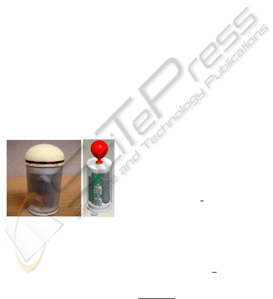
trol up to a depth of 150 feet. A prototype of the cylin-
drical shaped (1 liter in volume) membrane controlled
drogue is shown in Figure 1.
(a) (b)
Figure 1: Pneumatic membrane controlled cylindrical
shaped (a) drogue. Schematic inside view (b) of cylindri-
cal shaped drogue.
Similar flexible membranes for pneumatic con-
trol of underwater drogues have also been used in
ARGO floats (Gould, 2003; Gould, 2004), but at a
much larger form factor. In these design concepts,
the membrane actuation is primarily used for provid-
ing the buoyancy control for surfacing of the drogues.
Instead, to conform to a small form factor design,
we use the displaced volume under the flexible mem-
brane for both buoyancy control and the opportunity
to create alternating depth profiles that includes pe-
riodic surfacing. Due to the compressibility of the
membrane, the slightest perturbation in depth will
cause a change in volume and the equilibrium state
of the drogue is unstable. This is beneficial for low
energy periodic surfacing control. As shown in this
paper, feedback control can be used to stabilize the
drogue to any desired depth.
3 DYNAMIC MODELING OF
PNEUMATIC DROGUE
3.1 Rigid Body Dynamics
Assuming a drag parameter d due to a drag force in
water, the depth x(t) of the drogue can be described
by the second order differential equation
m¨x(t) + sign( ˙x(t))d ˙x
2
(t) = F
g
−F
b
(t) (1)
where the constant rigid mass of the drogue and added
mass due to displacement of fluid (Brennen, 1982) are
combined in the mass parameter m. In the equation
(1), F
g
is the downward (constant) gravitational force
F
g
= mg
and F
b
(t) is buoyancy force
F
b
(t) = ρg[V
b
(t) +V]
determined by the fixed drogue volume V and the dis-
placed volume V
b
(t) under the membrane. The con-
stant ρ is the density of the water, which we assume to
be constant at different depths. The drag parameter d
is determined by the drag coefficient c
d
of the drogue
moving in water at a low Reynolds number and typi-
cally given by
d =
1
2
c
d
ρA
where A denotes the frontal aerial surface of the
drogue. In the above equations, we consider V
b
(t) as
a control variable to control the depth of the drogue
using measurements of the depth x(t).
The condition of natural buoyancy at any depth
c ≥0 is determined by the initial conditions x(0) = x
0
and ˙x(0) = 0 for the differential equation given in (1)
and yields the desired (initial) volume
V
b
(0) = V
0
=
m
ρ
−V (2)
for natural buoyancy. Ideally, the mass m and the vol-
ume V of the drogue should be chosen to allow for a
Water density does depend on salidity and depth, but
these second order effects are neglected here
ICINCO 2010 - 7th International Conference on Informatics in Control, Automation and Robotics
90

large range in V
b
(t) > 0 for buoyancy control. How-
ever, even small changes in V
b
(t) suffice in generat-
ing motion of the drogue due to no-friction free body
movement of the drogue floating in water.
3.2 Actuator Dynamics
Using a pneumatic mechanism to add or bleed air
to effectively increase V
b
(t) induces additional (ac-
tuator) dynamics that needs to be taken into account
in order to design a control algorithm. The dis-
placed volume V
b
(t) under the membrane is a func-
tion of both the air flow, the stiffness of the membrane
and the external pressure surrounding the membrane.
Considering a flow φ(t) used to change the volume
V
b
(t) under the membrane, with the ideal gas equa-
tion (Fox et al., 2004) we see that the product of the
membrane pressure P
b
(t) and volumeV
b
(t) can be de-
scribed by
P
b
(t)V
b
(t) =
n
0
+
Z
t
τ=0
φ(τ)dτ
RT(t) (3)
where n
0
indicates the number of gas molecules for
natural buoyancy at t = 0, R is the Boltzman constant
and T(t) is the gas temperature which we assume to
be known (measurable) for now. Finally, we assume
a linear increase of the membrane pressure P
b
(t) due
to changes in the volume V
b
(t) according to
P
b
(t) = k
m
V
b
(t) + P
x
(t), P
x
(t) = k
x
x(t) + P
0
(4)
where k
m
is the (linear) membrane membrane stiff-
ness and P
x
(t) models the effect of the external pres-
sure as the sum of the atmospheric pressure P
0
and
the product of the depth x(t) and the pressure depth
constant k
x
given by
k
x
= ρg
The last equation allows us to compute the unknown
n
0
in (3) at time t = 0 for which we have natural buoy-
ancy and φ(0) = 0. With the desired initial displace-
ment volume V
0
under the membrane given in (2), we
see that at an initial depth x(0) = x
0
> 0
P
b
(0) = k
m
V
0
+ k
x
x
0
+ P
0
, V
0
=
m
ρ
−V
allowing us to compute n
0
as
n
0
=
k
m
RT
0
V
2
0
+
k
x
x
0
+ P
0
RT
0
V
0
, V
0
=
m
ρ
−V
indicating quadratic dependency on the initial dis-
placed volume V
0
under the membrane due to the lin-
ear membrane stiffness k
m
and linear dependency due
to influence of the depth dependent pressure.
To complete the analysis, we still need an equa-
tion that describes the flow φ(t). To anticipate the
switching control proposed in this paper, the flow φ(t)
is modulated by three different switching states: in-
flate, deflate or none. The input u can switch between
the values
u =
1 inflate
−1 deflate
0 none
can be used to distinguish between three different
switching states. Using the Bernoulli equation (Fox
et al., 2004) and assuming a steady incompressible
flow, each state has a different flow φ(t) that is mod-
eled via a proportional relationship with the square
root of the pressure difference:
φ(t) =
k
i
v
q
P
CO
2
−P
b
(t) u = 1
−k
d
v
p
P
b
(t) −P
x
(t) u = −1
0 u = 0
where P
CO
2
denotes the (constant) output pressure of
theCO
2
pressure regulator and k
i
v
, k
d
v
denote the valve
constants of respectively the add and bleed valves. If
both valves are the same, then k
v
= k
i
v
= k
d
v
. With the
pressure relationship given in (4) we see that the gas
flow φ(t) can now be modeled as
φ(t) =
k
i
v
q
P
CO
2
−k
x
x(t) −k
m
V
b
(t) −P
0
−k
d
v
p
k
m
V
b
(t)
0
(5)
respectively for u = 1, u = −1 and u = 0. As a result,
membrane inflation and deflation will occur at dif-
ferent flow rates. Membrane inflation is determined
mainly by the CO
2
pressure regulator, but pressure
build up due to depth and membrane stiffness (vol-
ume) has a negative influence. For deflation it can
be seen that only the membrane stiffness contributes
to a desired pressure difference and is independent of
depth.
3.3 Combined Dynamic Model
Combing the different equations and eliminating in-
termediate variables leads to a dynamic switching
system described by a set of coupled non-linear and
non-stiff ordinary differential equations (Hairer et al.,
1993) in depth x(t), volume V
b
(t) and gas flow φ(t)
given by
¨x(t) = −sign(˙x(t))
d
m
˙x
2
(t) +
ρg
m
(V
0
−V
b
(t))
k
m
V
b
(t)
2
+ [k
x
x(t) + P
0
]V
b
(t) =
n
0
+
Z
t
τ=0
φ(τ)dτ
RT(t)
DYNAMIC MODELING AND PNEUMATIC SWITCHING CONTROL OF A SUBMERSIBLE DROGUE
91

φ(t) =
k
i
v
q
P
CO
2
−k
x
x(t) −k
m
V
b
(t) −P
0
u = 1
−k
d
v
p
k
m
V
b
(t) u = −1
0 u = 0
where a summary of the meaning of the physical pa-
rameters is given in Table 2 in the Appendix of this
paper. For analysis purposes, the above dynamical
model is written in a short hand notation
˙z(t) = f
u
(z(t)) (6)
where z(t) = [x(t) ˙x(t) φ(t)]
T
combines the state vari-
ables and f
u
(z) for u ∈{ −1,0, 1}denotes the different
dynamic behavior of the system as a function of the
switching signal u. Simulations of the dynamics can
be done along with the initial conditions
z(0) =
x(0)
˙x(0)
φ(0)
=
x
0
0
0
and the resulting initial number of gas molecules n
0
and volume given V
0
by
n
0
=
k
m
RT
0
V
2
0
+
k
x
x
0
+ P
0
RT
0
V
0
V
0
=
m
ρ
−V
(7)
It can be observed from the above equations that the
membrane gas temperature T or density parameter ρ
can be considered as a time or depth varying param-
eters that influences the dynamics of the system. The
switching signal u ∈ {−1,0,1} is the control input
signal available to provide depth tracking and stabi-
lization for the drogue.
4 EQUILIBRIUM AND
STABILITY ANALYSIS
Equilibrium conditions for the drogue can be studied
by setting the flow rate φ(t) = 0 and the switching
signal u = 0, reducing the differential equations to
¨x(t) = −sign( ˙x(t))
d
m
˙x
2
(t) +
ρg
m
(V
0
−V
b
(t))
k
m
V
b
(t)
2
+ [k
x
x(t) + P
0
]V
b
(t) = n
0
RT(t)
(8)
Due to the assumptions of an ideal gas and lin-
ear membrane stiffness k
m
, the volume V
b
(t) can be
solved explicitely from the resulting quadratic equa-
tion as a function of depth x(t) and temperature T(t).
This yields a single solution under the constraint
V
b
(t) > 0 given by
V
b
(t) = −
1
2k
m
[k
x
x(t) + P
0
]+
1
2k
m
q
[k
x
x(t) + P
0
]
2
+ 4k
m
n
0
RT(t)
(9)
With T(t) = T
0
and both x(t), V
b
(t) > 0 and n
0
given
in (7) it can be seen that the solution
x(t) = x
0
> 0
˙x(t) = 0
V
b
(t) = V
0
=
m
ρ
−V > 0
is a stationary point of the equation in (8) as V
b
(t)
satisfies
−
1
2k
m
[k
x
x
0
+ P
0
]+
1
2k
m
q
[k
x
x
0
+ P
0
]
2
+ 4k
2
m
V
2
0
+ 4k
m
(k
x
x
0
+ P
0
)V
0
=
−
1
2k
m
[k
x
x
0
+ P
0
]+
1
2k
m
q
(2k
m
V
0
+ [k
x
x
0
+ P
0
])
2
= V
0
known as neutral buoyancy of the drogue at depth x
0
.
However, the stationary point is an unstable equilib-
rium as any perturbation on x(t) = x
0
causes an un-
bounded x(t), physically indicating that the drogue
will either surface or sink without control. Such dy-
namic behavior is due to the compressibility of the
membrane and can be used favorably to surface with-
out little or no control energy.
The instability of the equilibrium can be shown
by considering a perturbation on the depth x(t) > 0 at
time t = t
p
given by ¨x(t
p
) = 0 and x(t
p
) = x
0
+ ε, ε >
0. Due to this small increase in depth,
V
b
(t
p
) = −
1
2k
m
[k
x
(x
0
+ ε) + P
0
]+
1
2k
m
q
[k
x
(x
0
+ ε) + P
0
]
2
+ 4k
m
n
0
RT
0
= −
1
2k
m
[k
x
x
0
+ P
0
] −
1
2k
m
k
x
ε+ δ
where δ is given by the expression
1
2k
m
q
[k
x
x
0
+ P
0
]
2
+ 4k
m
n
0
RT
0
+ k
2
x
ε
2
+ 2k
x
(k
x
x
0
+ P
0
)ε
With 4k
m
n
0
RT
0
> 0, the strict inequality
δ <
s
q
[k
x
x
0
+ P
0
]
2
+ 4k
m
n
0
RT
0
+ k
x
ε
2
where
s
q
[k
x
x
0
+ P
0
]
2
+ 4k
m
n
0
RT
0
+ k
x
ε
2
=
=
q
[k
x
x
0
+ P
0
]
2
+ 4k
m
n
0
RT
0
+ k
x
ε
indicates that
V
b
(t
p
) < −
1
2k
m
[k
x
x
0
+ P
0
]+
1
2k
m
q
[k
x
x
0
+ P
0
]
2
+ 4k
m
n
0
RT
0
= V
0
ICINCO 2010 - 7th International Conference on Informatics in Control, Automation and Robotics
92

making the displaced volume V
b
(t
p
) under the mem-
brane smaller than V
0
due to x(t
p
) = x
0
+ ε. With
(V
0
−V
b
(t
p
)) > 0 and ¨x(t
p
) = 0, the differential equa-
tion for x(t) in (8) indicates ˙x(t
p
) > 0 causing a further
increase of the depth x(t) for t > t
p
. This indicates
the increase of the depth x(t) (sinking) and the insta-
bility of the neutral buoyancy operating point of the
drogue at x(t) = x
0
. A similar argument can be given
for a perturbation x(t
p
) = x
0
−ε that will result in a de-
crease in the displaced volume V
b
(t
p
) under the mem-
brane, causing the drogue to surface. The stability
analysis indicates that neutral buoyancy is obtained
only at one specific (initial) depth x
0
such that V
b
(t)
given in (9) satisfies V
b
(t) = V
0
= m/ρ−V to provide
a buoyancy force that balances the gravitational force.
5 DEPTH SWITCHING
CONTROL
Although the compressibility of the membrane can be
used favorably to surface or sink the drogue without
little or no control energy, a contraction or stabiliza-
tion algorithm towards a target depth reference r(t)
must be implemented via feedback control. Due to the
switching behavior of the control signal u∈{−1, 0,1}
we can only expect to obtain depth tracking and neu-
tral buoyancy within a user specified tolerance level
α around the depth reference r(t). Our objective is to
design a switching control algorithm that guarantees
attaining the depth region |x(t) −r(t)| < α from an
arbitrary initial depth condition x
0
.
In this paper this is achieved by simply modulat-
ing the switching signal u ∈ {−1,0,1} on the basis of
feedback information of the depth x(t) and the depth
velocity ˙x(t). With a target depth r(t) > 0 and a γ
with 0 < α < γ, the depth measurements are classified
in three different regions that are pairwise disjoint
R
1
= {x | γ < |r(t) −x|}
R
2
= {x | α < |r(t) −x| ≤ γ}
R
3
= {x | |r(t) −x| ≤ α}
(10)
respectively denoted by the attraction region R
1
, the
stabilization region R
2
and the tolerance region R
3
.
We will first summarize the proposed switching con-
trol algorithm. Subsequently we provide a proposi-
tion that shows how contraction to a specific depth
region can be obtained.
Algorithm 1. Let R
j
, j = 1, 2,3 be the depth region
defined in (10) where 0 < α < γ and consider the max-
imum drogue velocities β
j
for each region R
j
where
β
3
≤ β
2
≤ β
1
and let
σ = sign(r(t) −x(t)) ∈ {−1,1}
Default, the switching signal u = 0 but will be either
u = 1 (add air to increase the volumeV
b
(t)) or u = − 1
(bleed air to reduce V
b
(t)) according to the following
rules:
1. If x(t) ∈R
1
, consider the two situations:
a. If |˙x(t)| ≤ β
1
then u = −σ (increase depth ve-
locity)
b. If σ · ˙x(t) < 0 then u = −σ (velocity in wrong
direction, increase/decrease depth velocity di-
rectly)
2. If x(t) ∈R
2
, consider the two situations:
a. If |˙x(t)| > β
2
and σ · ˙x(t) > 0 then u = σ (de-
crease velocity)
b. If σ · ˙x(t) < 0 then u = −σ (velocity in wrong
direction, increase/decrease depth velocity di-
rectly)
3. If x(t) ∈ R
3
and |˙x(t)| > β
3
then u = sign{˙x(t)}
(chatter input signal to achieve velocity bound)
As can be seen from the above algorithm, each
region R
j
, j = 1,2,3 has specific bounds β
j
on the
depth velocity ˙x(t) that determines the modulating of
the switching signal u ∈ {−1,0,1}. The attraction re-
gion R
1
is used to give the drogue the right velocity
with a maximum of β
1
to attract it in the stabilization
region R
2
. When the drogue enters the region R
2
, the
velocity is reduced to β
2
to avoid abrupt entering and
exiting of R
2
and providing an entering velocity of
β
2
for the tolerance region R
3
. Obviously, the choice
of β
2
is closely related to the size of γ. As soon as
the drogue enter the tolerance region R
3
the control
can be turned off by choosing β
3
= β
2
as the entering
velocity will be β
2
. Choosing β
3
< β
2
allows an ad-
ditional reduction of drogue velocity within the toler-
ance region at the price of a chattering control signal.
The proposed switching control in Algorithm 1 is
motivated by the need to dampen the (unstable) rigid
body motion of the drogue and maintain neutral buoy-
ancy. The proposed algorithm is basically a Propor-
tional and Derivative (PD) control architecture with
specific level sets for position x(t) and velocity ˙x(t)
measurements. It should be observed that feedback
information on x(t) and ˙x(t) is required to implement
the proposed control algorithm. However, ˙x(t) can
be approximated by discrete-time sampling and filter-
ing of the depth x(t), allowing a discrete-time imple-
mentation of the switching control algorithm based on
depth measurements only.
DYNAMIC MODELING AND PNEUMATIC SWITCHING CONTROL OF A SUBMERSIBLE DROGUE
93
6 HYBRID STABILITY ANALYSIS
For the analysis of the proposed switching control
algorithm, the framework of hybrid systems analy-
sis (Van der Schaft and Schumacher, 2000; Liberzon,
2003; Goebel et al., 2009) can be used to prove stabil-
ity properties of the resulting control system. Based
on the switching control law proposed in Algorithm 1,
the behavior of the drogue is modeled as a hybrid sys-
tem with three different modes corresponding to in-
flation for u = 1, deflation for u = −1, and a neutral
mode for u = 0.
Each mode has its active region and these regions
share switching surfaces with each other. The tran-
sition between modes occurs when the system trajec-
tory crosses these switching surfaces. In this paper,
a multiple Lyapunov functions based parameter de-
pendent switching strategy is used to investigate the
stability of the proposed switching control algorithm
for the buoyancy control of the drogue.
In order to establish an active region for each actu-
ator dynamic mode, three Lyapunov functionsV
u
, u ∈
{−1, 0,1} must be defined. The three quadratic Lya-
punov functions V
u
are defined as follows:
V
1
=
1
2
(−(x−r) −10˙x+ φ)
2
inflation
V
−1
=
1
2
(−(x−r) −10˙x+ φ)
2
deflation
V
0
=
1
2
(x−r)
2
+
1
20
˙x
2
neutral
(11)
Subsequently, the stability analysis is based on a the-
orem in (Branicky, 1998) on Lyapunov stability of
switched and hybrid systems and summarized in the
following result for the switched hybrid system con-
sidered in this paper.
Proposition 1. Consider the system ˙z(t) = f
u
(z(t)) in
(6) and let V
u
be the Lyapunov functions given in (11)
for u ∈ {−1, 0,1}. Let L
f
u
V
u
be the Lie derivative
of V
u
along the vector field spanned by the subsystem
f
u
(·). The origin of the system is asymptotically stable
if the following two conditions are satisfied
(a) L
f
u
V
u
< 0 for each u ∈ {−1,0,1}
(b) V
u
is nonincreasing along switching
times on the uth system ˙z(t) = f
u
(z(t))
(12)
In this paper we use numerical analysis to ver-
ify the two conditions (12) in Proposition 1. It can
be verified that each Lyapunov function V
u
for u ∈
{−1, 0,1}in (11) is positive definite over its active re-
gion characterized by L
f
u
V
u
< 0. To characterize (12)
over the three dimensional state vector z = [x ˙x φ]
T
Lyapunov analysis is conducted by varying φ in the
admissible range. This can be done as φ is not used
directly in the switching control of Algorithm 1. Nu-
merical evaluation of (12) for different values of φ
is done using a non-stiff differential equation solver
(Cooper, 2004) and implemented via
ode45
in Mat-
lab.
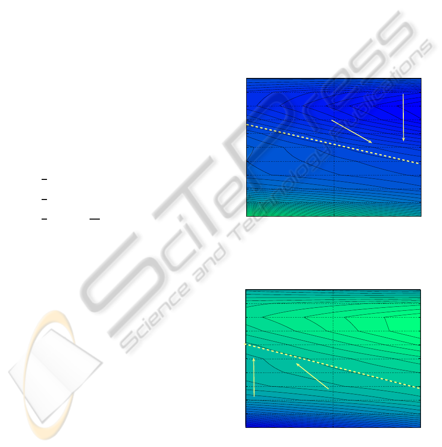
For the inflation mode, L
f
1
V
1
for φ = 0 is plotted
in Figure 2 and the active region for which (12) holds
is separated by a dashed line, whereas the arrows indi-
cate a decreasing value of V
1
. If φ is varied, the whole
solution surface moves through the φ-axis (perpendic-
ular to x− ˙x plane) resulting in the shift of the active
region along the ˙x-axis. The same analysis can be
done for other modes. A similar plot is created for the
deflation mode where L
f
−1
V
−1
for φ = 0 is plotted in
Figure 3 and the neutral mode where L
f
0
V
0
for φ = 0
is plotted in Figure 4.
Depth
Velocity
r
−0.5
−0.4
−0.3
−0.2
−0.1
0
0.1
0.2
0.3
0.4
0.5
L
f1
V
1
<0 (active region)
L
f1
V
1
>0
Figure 2: The active region of the inflation mode. The ar-
rows indicate the allowable direction of solution trajectory.
In inflation mode, the solution trajectory always follows this
allowable direction.
Depth
Velocity
r
−0.5
−0.4
−0.3
−0.2
−0.1
0
0.1
0.2
0.3
0.4
0.5
L
f−1
V
−1
<0 (active region)
L
f−1
V
−1
>0
Figure 3: The active region of the deflation mode. The ar-
rows indicate the allowable direction of solution trajectory.
In deflation mode, the solution trajectory always follows
this allowable direction.
ICINCO 2010 - 7th International Conference on Informatics in Control, Automation and Robotics
94
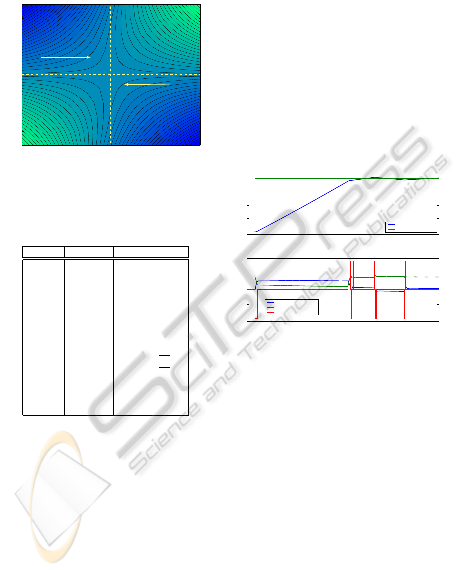
Depth
Velocity
r
−0.5
−0.4
−0.3
−0.2
−0.1
0
0.1
0.2
0.3
0.4
0.5
L
f0
V
0
<0
(active region)
L
f0
V
0
<0
(active region)
L
f0
V
0
>0
L
f0
V
0
>0
Figure 4: The active region of the neutral mode. The ar-
rows indicate the allowable direction of solution trajectory.
In neutral mode, the solution trajectory always follows this
allowable direction.
Table 1: Numeric parameters of dynamic drogue model for
non-linear simulation of switching control algorithm.
symbol value units
V 10
−3
m
3
m 1.5 kg
d 30 N/m
2
/s
2
ρ 1.03·10
3
kg/m
3
g 9.81 m/s
2
k
m
5·10
8
Pa/m
3
or N/m
5
T
0
288 K
R 8.314472 (m
3
Pa)/(K mol)
k
a
10
−4
mol/
√
Pa
k
b
10
−4
mol/
√
Pa
P
CO
2
10
6
Pa or N/m
2
P
0
10
5
Pa or N/m
2
x
0
10 m
Based on these figures, the existence of a stability
region characterized by (12) can be verified. There-
fore, the proposed hybrid control strategy using the
active regions and switching surfaces stabilizes the
drogue system.
7 SIMULATION RESULTS
To illustrate the performance of the switching control
in Algorithm 1, the controlled dynamic behavior of a
model of a buoyancy controlled submersible drogue
is simulated. The model is based on the set of cou-
pled non-linear differential equations given in (6) and
based on the numerical parameters listed in Table 1.
A summary of the meaning of the physical parameters
is given in Table 2 in the Appendix of this paper.
Using the switching control summarized in Algo-
rithm 1 with the regions of (10) based on a depth toler-
ance α = 0.5m and a stabilization region specified by
γ = 2α = 1m and a maximum velocity β
1
= 0.3m/s in
region R
1
and a maximum velocity β
2
= β
3
= 0.1m/s
in region R
2
and R
3
, the performance of the switching
control algorithm can be evaluated by the simulation
results depicted in Figure 5. The results were com-
puted by numerically solving the non-stiff differential
equations of the ODE’s of the model of the drogue
using an implementation of the explicit Runge-Kutta
(4,5) pair implemented in
ode45
in Matlab (Shampine
and Reichelt, 1997).
0 20 40 60 80 100 120
10
15
20
25
30
Result of closed−loop (full state feedback) simulation of drogue
depth [m]
reference depth [m]
0 20 40 60 80 100 120
−1
−0.5
0
0.5
1
time [sec]
depth velocity [m/s]
bladder volume [liter]
control input [−1,0,1]
Figure 5: Simulation results of switching control Algo-
rithm 1 with α = 0.5m, γ = 1m, β
1
= 0.3m/s and β
2
=
β
3
= 0.1m/s when the target depth references r(t) changes
from 10m to 30m at t = 5sec. The numerical values for
the drogue model used during this simulation are listed in
Table 1.
During the simulation the target depth r(t) of 10m,
for which the drogue is initially neutrally buoyant, is
changed to 30m at t = 5sec. It can be seen from the
simulation results in Figure 5 that the drogue stays
within approximately ±αm of the a constant target
depth, whereas a change to a different target depth is
accomplished with a maximum speed of β
1
= 0.3m/s
and only requires a few switches of the control signal
u. During steady state operation only very short actu-
ation of either the ”add” (u = 1) or ”bleed” (u = −1)
valves are used to maintain depth within the speci-
fied tolerance region α and stabilization region γ. The
simulation confirms the hybrid stabilization results.
DYNAMIC MODELING AND PNEUMATIC SWITCHING CONTROL OF A SUBMERSIBLE DROGUE
95
8 EXPERIMENTAL RESULTS
In an initial testing phase, the proposed control al-
gorithm was implemented on the pneumatic mem-
brane controlled cylindrical shaped drogue depicted
in Figure 1(a). The drogue design uses an internally
stored standard compressed 16 gram CO
2
cartridge
with a regulator assembly to change the displaced vol-
ume under the latex or neopropene membrane via two
small form factor Numatics series solenoid valves.
One valve is used for inflating the membrane, the
other valve is to bleed the CO
2
from the membrane.
The electrical components are powered by three
3.7Volt, 2700mAH Li-Ion batteries. A model 85 Ul-
tra Stable Pressure Sensor is used for depth measure-
ments measured by a 10bit AD converter on a Mi-
crosystems PIC18F4620 microprocessor.
The embedded control of the pneumatically con-
trolled drogue only uses depth measurements x(t)
sampled at 10Hz and depth velocity estimates v(t) are
obtained via
v(t) =
x
f
(t) −x
f
(t)
∆
t
, x
f
(t) = F(q)x(t)
where F(q) is a second order Butterworth filter with
a normalized cut-off frequency of 0.1 (1Hz). Both the
depth measurements x(t) and the control signal u(t)
as a function of the discrete-time t were saved for val-
idation purposes and the results of the experimental
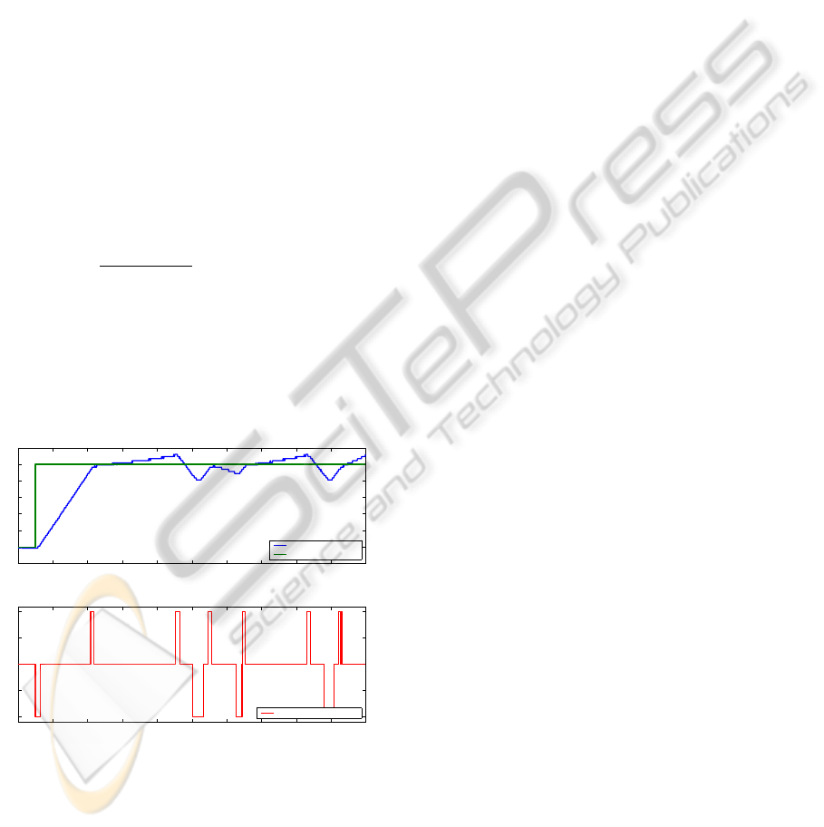
work is summarized in Figure 6.
0 10 20 30 40 50 60 70 80 90 100
9
10
11
12
13
14
15
16
0 10 20 30 40 50 60 70 80 90 100
−1
−0.5
0
0.5
1
time [sec]
depth [m]
reference depth [m]
switching control signal
Figure 6: Preliminary experimental results of switching
control Algorithm 1 with α = 0.5m, γ = 1, β
1
= 0.3m/s and
β
2
= β
3
= 0.2m/s applied to the pneumatic membrane con-
trolled cylindrical shaped drogue depicted in Figure 1(a).
The target depth references r(t) changes from 10m to 15m
at t = 5sec.
The experimental results confirm the stability of
the control algorithm for the pneumatic membrane
cylindrical shaped drogue even for the discrete-time
implementation of the algorithm. The slightly larger
values of β
2
and β
3
, chosen due to the noise lev-
els on the estimated velocity v(t), cause larger ve-
locity swings in the stabilization and tolerance re-
gion. Moreover the quantization effects of the depth
measurements based on a 10bit AD converter also
cause resolution limiations on the velocity estimate.
It can be seen that a larger value for β
2
requires more
switching for stabilization. Tuning of the controller
parameters α, γ, β
1
and β
2
can be used to further im-
prove the controller performance.
9 CONCLUSIONS
The dynamic properties of a submersible drogue for
which buoyancy control is implemented by a flexible
membrane can be described by a set of coupled non-
linear and non-stiff ordinary differential equations. It
is shown that the compressibility of the membrane
leads to an dynamically unstable dynamical system
in terms of the depth, which can be used favorably to
surface or sink the drogue without little or no control
energy.
The instability does require a contraction or sta-
bilization algorithm to maintain a target depth refer-
ence. In this paper it is shown that a simple pneu-
matic on/off switching control algorithm in which
compressed CO
2
is either added or extracted from the
membrane actuator on the basis of three different and
pairwise disjoint depth regions can be used to stabi-
lize the depth positioning of the drogue.
The switching control algorithm leads to a hybrid
dynamical system, for which stability analysis results
are summarized in the paper. Numerical evaluation
of the stability conditions reveal that the proposed
on/off switching control algorithm leads to a stabi-
lized buoyancy-controlled drogue. Both simulation
and experimental studies indicate stability properties
and depth tracking performance within a specified tol-
erance levels.
REFERENCES
Bhatta, P., Fiorelli, E., Lekien, F., Leonard, N. E., Paley, D.,
Zhang, F., Bachmayer, R., Davis, R. E., Fratantoni,
D. M., and Sepulchre, R. (2005). Coordination of an
underwater glider fleet for adaptive ocean sampling.
In International Workshop on Underwater Robotics,
Int. Advanced Robotics Programmed (IARP), Genoa,
Italy.
Branicky, M. (1998). Multiple Lyapunov functions and
other analysis tools for switched and hybrid systems.
ICINCO 2010 - 7th International Conference on Informatics in Control, Automation and Robotics
96

IEEE Transactions on Automatic Control, 43:475–
482.
Brennen, C. (1982). A review of added mass and fluid in-
ertial forces. Technical Report CR82.010, Naval Civil
Engineering Laboratory.
Colgan, C. (2006). Underwater laser shows. Explorations,
Scripps Institution of Oceanograhpy, 12:20–27.
Cooper, J. (2004). An Introduction to Ordinary Differential
Equations. Cambridge University Press.
Davis, R. (1991). Observing the general circulation with
floats. Deep-Sea Research, 38:531–571.
Fiorelli, E., Bhatta, P., Leonard, N. E., and Shulman, I.
(2003). Adaptive sampling using feedback control of
an autonomous underwater glider fleet. In Proceed-
ings 13th International Symposium on Unmanned Un-
tethered Submersible Technology, Durham, NH.
Fox, R., McDonald, A., and Pritchard, P. (2004). Intro-
duction to Fluid Mechanics. John Wiley & Sons Inc.,
Hoboken, NJ, U.S.A.
Goebel, R., Sanfelice, R. G., and Teel, A. R. (2009). Hybrid
dynamical systems. IEEE Control Systems Magazine,
29:283.
Gould, J. (2004). Argo profiling floats bring new era of in
situ ocean observations. Earth and Ocean Sciences,
85(11).
Gould, W. J. (2003). WOCE and TOGA - the foundations
of the global ocean observing system. Oceanography,
Special Issue on Ocean Observations, 16(4):24–30.
Hairer, E., Nørsett, S. P., and Wanner, G. (1993). Solving
Ordinary Differential Equations I: Nonstiff Problems.
Springer Verlag, Berlin.
Helfrich, K. and White, B. (2007). Rapid gravitational
adjustment of a horizontal shear layer. In American
Physical Society, 60th Annual Meeting of the Divison
of Fluid Dynamics.
Kunzig, R. (1996). A thousand diving robots. Dis. Mag.,
17:60–63.
Liberzon, D. (2003). Switching in Systems and Control.
Systems & Control: Foundations and Applications se-
ries. Birkhauser, Boston.
Ly, L. N. and Luong, P. (1997). A mathematical coastal
ocean circulation system with breaking waves and nu-
merical grid generation. Applied Mathematical Mod-
elling, 21:633–641.
Paley, D., Zhang, F., and Leonard, N. E. (2008). Cooper-
ative control for ocean sampling: The glider coordi-
nated control system. IEEE Transactions on Control
Systems Technology, 16:735–744.
Perry, M. and Rudnick, D. (2003). Observing the ocean
with autonomous and lagrangian platforms and sen-
sors (ALPS): The role of ALPS in sustained ocean
observing systems. Oceanography, 4:31–36.
Schofield, O. and Tivey, M. (2004). Building a window to
the sea: Ocean research interactive observatory net-
works (ORION). Oceanography, pages 113–120.
Shampine, L. F. and Reichelt, M. W. (1997). The Matlab
ODE suite. SIAM Journal on Scientific Computing,
18:1–22.
Van der Schaft, A. and Schumacher, H. (2000). An Intro-
duction to Hybrid Dynamical Systems. Lecture Notes
in Control and Information Sciences 251, Springer-
Verlag.
APPENDIX
Table 2 summarizes the symbols use in the derivation
of the dynamical model of the drogue in Section 3.3.
Table 2: Summary of symbolic parameters of dynamic
drogue model.
symbol meaning
V volume of drogue
m mass of drogue
d drag parameter in water
ρ density of sea water
g gravitational constant
k
m
linear membrane stiffness
T
0
temperature of water
R gas constant
k
a
‘add air’ valve constant
k
b
‘bleed air’ valve constant
P
CO
2
regulated CO
2
pressure
P
0
atmospheric pressure
x
0
depth for neutral buoyancy
DYNAMIC MODELING AND PNEUMATIC SWITCHING CONTROL OF A SUBMERSIBLE DROGUE
97
