
ATC
An Asymmetric Topology Control Algorithm for Heterogeneous Wireless Sensor
Networks
Mohsen Nickray and Ali Afzali-kusha
Low-Power High-Performance Nanosystems Laboratory
Department of Electrical and Computer Engineering, University of Tehran, Tehran, Iran
Keywords: Wireless sensor network, Power control, Asymmetric topology control.
Abstract: In this paper, we present an asymmetric topology control (ATC) algorithm for wireless sensor networks. In
this algorithm, the sensor nodes incrementally adjust their transmission. The algorithm had three phases of
Neighbor Discovery, Construct Topology, and Data Transmission. In the phase of Neighbor Discovery, the
nodes exchanged their positions and maximum transmission powers. In phase II, each sensor node
collaboratively adjusted its transmission range (power) while keeping the network connectivity the same as
that of the case of transmitting with the maximum power. In phase III, all the nodes transmit data with the
adjusted transmission power. To assess the efficiency of the proposed algorithm, its performance is
compared to those of previously published works. Our algorithm not only preserve power and average node
degree and average link length, it has privileges which enable it to work properly even in the absence of
conventional error handling mechanisms.
1 INTRODUCTION
Recent advances in wireless and electronics
technologies have led to emergence of wireless
sensor networks (WSN) with large scale nodes.
They are used in a wide spectrum of applications
including industrial, military, and health monitoring
applications. Most of these devices have limited
battery lifetime where after depletion, it is extremely
difficult (if not impossible) to replace the batteries.
As a result, WSNs need efficient mechanisms which
minimize the energy consumption while maintaining
the network connectivity and improving the network
capacity which is the simultaneous data transfer rate.
The topology control determines the required
transmission power of each node to maintain the
network connectivity while the energy consumption
is minimized. Instead of transmitting with a
maximum power, nodes in a wireless network
collaboratively determine their transmission power
and derive the network topology by forming proper
neighbor relations under a specific topology control
algorithm (Narayanaswamy et al., 2002). Using
adjusted transmission power have several benefits
(Rodoplu and Meng, 1999). They include
minimizing the MAC layer contention, improving
the spatial reuse and network capacity, and
increasing the network life time by minimizing the
power consumption.
WSNs are divided into two categories of
homogeneous and heterogeneous. The homogeneous
network contains devices with the same hardware
capabilities such as computation, link, energy, and
communication range while the heterogeneous
network includes devices with different hardware
capabilities. Note that the heterogeneity in the
transmission range of the nodes leads to asymmetric
links where the transmission and receive paths are
not the same. Asymmetric links are normally
unidirectional. Recently in the literature,
heterogeneous WSNs have attracted more attention.
In these networks, asymmetric protocols seem
unavoidable for two reasons (Liu and Li, 2003).
Firstly, if all the links in the original topology are
symmetric, it is not possible to assume different
transmission ranges among nodes. In this case, the
two farthest neighbors in network determine the
transmission power of all the nodes. Secondly, if
asymmetric links are allowed to exist in the finalized
topology, the derived minimum power topology may
become more power-efficient since the transmission
range for each node may be determined according to
the situation of its neighbors.
75
Nickray M. and Afzali-kusha A. (2010).
ATC - An Asymmetric Topology Control Algorithm for Heterogeneous Wireless Sensor Networks.
In Proceedings of the Inter national Conference on Wireless Information Networks and Systems, pages 75-81
DOI: 10.5220/0002984800750081
Copyright
c
SciTePress

In this paper, we consider the heterogeneity of
the communication range for the WSN nodes. We
introduce a distributed algorithm which constructs a
topology with asymmetric links. In the algorithm,
the information is only exchanged between the
nodes which are attributed as local neighbors. As the
algorithm is localized, it could be applied to
networks with large scales. The rest of the paper is
organized as follows. In Section II, we briefly
review some related works on the topology control
and the differences of this work with them are
discussed. The proposed algorithm is presented in
Section III. In Section IV, the results are discussed.
Finally, section V concludes the paper.
2 PREVIOUS WORKS
The concepts of relay region and enclosure for the
purpose of power control were presented in
(Rodoplu and Meng, 1999). The relay region is
defined based on the following property. If the node
i consumes less power when it chooses to relay
through the node r instead of transmitting directly to
node j, then the node j is in the relay region of node
r. The enclosure of the node i is then defined as the
union of the complement of the relay regions of all
the nodes that the node i can reach by using its
maximal transmission power. Although the proposed
technique generates an energy efficient topology, it
has a high messaging overhead (Rodoplu and Meng,
1999).
In (Li et al., 2003), a bidirectional topology
based on Minimum Spanning Tree is introduced.
The network connectivity is preserved in this
topology where the degree of each node is bounded
by six. A bounded degree is desirable because a
small node degree reduces the MAC level contention
and interference (Li et al., 2003). In (Li et al., 2001),
CBTC(α) which is a two-phase algorithm is
proposed. In this algorithm, each node finds the
minimum power p such that transmitting with it
guarantees that it can reach at least one node in
every cone of degree of α. It was analytically shown
that if α < 5π/6, the network connectivity will be
preserved.
A three phase algorithm for the topology control is
introduced in (Liu and Li, 2003). In the first phase,
each node broadcasts an initialization message
where the nodes in its vicinity reply with a message
containing their locations and maximum powers.
Based on the information, each node establishes its
vicinity graph. In the second phase, the minimum
power vicinity tree is derived from the vicinity graph
using the execution of the shortest path algorithm. In
the third phase, each node calculates its transmission
power and required transmission power of their
vicinities by running the shortest path algorithm, and
informs the neighbors using Power Request (PRQ)
Messages. Each node, when receives a PRQ
message from a neighbor, compares the power
requirement from the neighbor node with its current
power setting. If a neighbor requires a stronger
transmission power, the node increases its power
accordingly. The minimum-power topology
guarantees the same reachability between any two
nodes compared with the maximum topology where
the nodes use their maximum transmission powers.
The important shortcoming of the algorithm is its
vulnerability to the packet loss in the third phase.
PRQ losses lead to irreparable problems. Packet
losses may occur in WSNs for the reasons explained
here. Normally, WSNs are set up in adverse
environmental conditions, like wind and rain, where
the communication can be disrupted. In the
configuration steps of sensor networks, where there
is no topology control algorithm, all the nodes will
transmit using the maximum power, and hence,
packet losses are more probable.
Based on the above discussion, an asymmetric
algorithm resistant to the packet loss is desired. In
this paper, we introduce an asymmetric topology
control algorithm which overcomes the shortcoming
of the algorithm presented in (Liu and Li, 2003). The
proposed algorithm works properly when the packet
loss occurs but at a lower efficiency. In this paper
the efficiency is assumed as a function of the
average node degree and the average link length.
The efficiency of the algorithm degrades inversely
proportional to the packet loss rate.
3 PROPOSED ASYMMETRIC
TOPOLOGY CONTROL
ALGORITHM
The ATC algorithm which is proposed in this work
is shown in Fig. 1. It is a distributed and localized
algorithm which efficiently assigns the power level
of each sensor node. The goal of the algorithm is to
find a minimum transmission power of P
i
such that
the network connectivity is preserved. Algorithm has
three phases which include Neighbor Discovery,
Construct Topology, and Data Transmission.
A. Phase I
In the first phase, the node
broadcasts a discovery
Hello message. The message contains
,
and
WINSYS 2010 - International Conference on Wireless Information Networks and Systems
76

P
i
max
which are the location and maximum power of
the node using the maximum power of the node
which is P
i
max
. Having received this broadcast
message, each neighbor j replies to it by a message
which contains its location and maximum power
using its maximum power of P
j
max
. The node
detects the set of its localized neighbor denoted by
Ν
based on the received reply messages. The
node stores the neighbor unique ID nodes which is
determined in the link layer, in a maximum range
table (MRT) along with their other information
including their positions and maximum ranges based
on the received current power levels. The latter will
be adjusted in the second phase.
Ν
As mentioned before, the reply messages are
transmitted with P
j
max
. Even with this power level, if
the node
is not in the range of one of its
neighbors, it needs a multi hop path to reach
. This
may occur due to the fact that we have a
heterogeneous network with different transmission
ranges. Various mechanisms like re-broadcasting by
relay nodes, sending the message via network layer
packet routing protocols, or using sub-routing layer
services could be used (Liu and Li, 2003).
B. Phase II
In the Construct Topology phase, each node n
i
should decide about its final transmission power
denoted by P
i
. The power is determined by a
distributed process stated in phase II of Algorithm1
shown in Fig. 1. Any change in the node power level
will be informed by broadcasting an update message
with the maximum power of P
i
max
. Each node
updates its MRT table using the update packets sent
by its neighbors. To determine the current
transmission power of the node i, the algorithm
starts by initializing the power to the amount needed
to reach the nearest neighbor in
. Then, each
node incrementally adjusts the power such that it
achieves the same neighbor set as the maximum
range topology.
In phase II of the algorithm, in order to construct
the final topology of
, we need
|
Ν
|
1
iterations. The final topology will contain the least
possible number of edges which is equal to
|
|
1.
In each iteration, the algorithm wait for new update
messages before selecting a new edge. The wait time
is controlled by a timer denoted by T
i
. If during the
timer interval of T
i
, a broadcast message is received
from a neighbor in
, then the MRT table and
are updated. In each iteration, the algorithm
should add one link. At the end of wait time, based
on the new MRT values,
-
is evaluated.
Figure 1: Algorithm 1 clarify the body of the ATC
algorithm.
Table 1: ATC algorithm notations.
symbol Definition
Current power level of node
Topology for the node n
i
resulted by
Algorithm2 including vertices (
) and edges (
) resulted from
MRT(
)
,
Topology for the node
n
i
resulted from ATC algorithm
including vertices (
) and
finalized edges
outward
edges
the edge from a closer neighbor to
farther neighbor edges
backward
edges
the edge from a farther neighbor to
closer neighbor
,
A directional edge from
(Source
node) to
(Destination node).
Phase I:
1 broadcast(
,
,
,
)
2 broadcast messa
g
e is received from all nei
g
hbors and
create
3
Phase II:
4
5
,
6 broadcast(
,
,
)
7 while (
|
T
|
|
|
1
8 {
9 update
10 set timer T
i
11 If ( broadcast message is received from a
neighbor before timer expires )
12 {
13 update MRTable
14 update
15 }
16 if (timer T
i
expires)
17 {
18 if (
|
|
1
19 {
20 calculate Δ
21
Δ
22 update MRT
23 update
24 broadcast(
,
)
25 }
26 }
27
= edge with minimum weight from
(
,T
)
28
29 }
31
32
Phase III
33 Transmit(
,Data, ,
)
ATC - An Asymmetric Topology Control Algorithm for Heterogeneous Wireless Sensor Networks
77

,
,
Noting that
is the number of edges before this
iteration, if G
-
, it means that we can add
a new edge to
. For this condition, Algorithm
2, which is given in Fig. 2, selects the edge with the
minimum distance. Otherwise (
-
), it
means that with the current power, we cannot add a
new edge and the power should be increased. For
this purpose,
is minimally incremented with ∆p
such that at least one new
,
edge denoted by
e
i
can be added to
. This edge is selected as a
new member for
and a update message is
transmitted to the neighbors, to be informed about
the last transmission power change.
Figure 2: Algorithm 2 which constructs
.
Algorithm2 (Update
) which is called by
Algorithm1 is used to construct
. This
algorithm generates an asymmetric local graph
(
,
) which contains all the feasible edges
based on the transmission ranges of the current
neighbors in the MRT table. Each edge in
has
the potential to be selected as
in line 28 of
Algorithm1. In lines 3-7 of Algorithm 2, the outward
edges and in lines are 8-14 the selection of backward
edges are checked. When the algorithm adds
outward edge
,
, line 5 checks
to see if it
is in the transmission range of
. Also, line 6
makes sure that none of the edges in T
has n
w
as
its destination node. In the addition of the backward
edges, the edge
,
is added when
is in the
range of
(line 10),
is accessible from
(line
11), none of the edges in T
has common
destination nodes with the
,
(line 12), and
the edge with reverse direction is not a member of
T
(line 13) (
,
T
. After
|
|
1 iterations,
which is an asymmetric topology
containing
|
|
1 directional edge is constructed.
C. Phase III
Phase III of the algorithm is Data Transmission.
While all the messages in phases I and II are
transmitted with the maximum power level, in phase
III all the messages will be transmitted with the
transmission power of
determined in Phase II.
D. Example for The Proposed Algorithm
Fig. 3 illustrates the results of running of the
proposed algorithm on node n
1
. In the first phase of
the algorithm, the node detects its neighbors and
constructs the MRT table. Phase II devotes to the
power adjustment. In phase II, firstly, r
1
is initialized
by 1 as the distance between n
1
and its nearest
neighbor and the edge (n
1
, n
2
) is added to
.
Figure 3 part (a) depicts topology for n1 after initial
part of phase II. Figure 3 part (b) shows all the
details happened in iteration 1. After the expiration
of timer T
1
, the MRT table is updated by the recent
update messages showing the determined power of
each node up to this iteration. For this example,
according to received update messages
((n2,1)(n3,2)(n4,2)) the transmission range of n
2
, n
3
,
and n
4
has updated to 1, 2, and 2, respectively. Note
that at this stage, the update messages of nodes n5
and n6 have not received by node 1. Finally
algorithm in this iteration select the edge with the
minimum weight which is (n
4
, n
7
). In iteration 2
(Fig. 3 part (c)), edge (n
3
, n
5
) is selected. In iteration
3 (Fig. 3 part (d)), after the timer expiration, we have
-
. Hence, the algorithm assumes
∆p
√
10 and add (n1, n4) to
. In iteration 4,
the MRT values lead the algorithm to select (n
7
, n
6
).
Part (e) of figure 3 depicts details of the iteration.
Finally, in the last iteration (figure 3 part (f)), n1
received (n2, 2) and update
and result will be
addition of (n2, n3) to the
. As figure shows
the algorithm clarify all the transmitted packets by
n1 for each iteration. n1 in phases I and II, totally
sends 3 messages which all the messages are
transmitted using maximum power.
E. Example for the Proposed Algorithm in
Presence of Packet Miss
In this part we assume some problems have been
suddenly happened in our network and the worst
possible scenario has happened: All the packets from
all the neighbors are damaged and we don’t have
any recovery mechanism then any one of our packets
Update
1
,
2 Sort all vertices in
in increasing order of distance
to
3 for (k=1 to
1)
4 for (w=k+1 to
|
|
)
5 if (
6 and there is not any ,
in Γ
that
x
)
7
,
8 for (k=
|
|
to 2)
9 for (w=k-1 to 1)
10 if (
11 and there is a path(
12 and there is not any ,
in T
that
x
13 and there is not
,
in T
)
14
,
WINSYS 2010 - International Conference on Wireless Information Networks and Systems
78
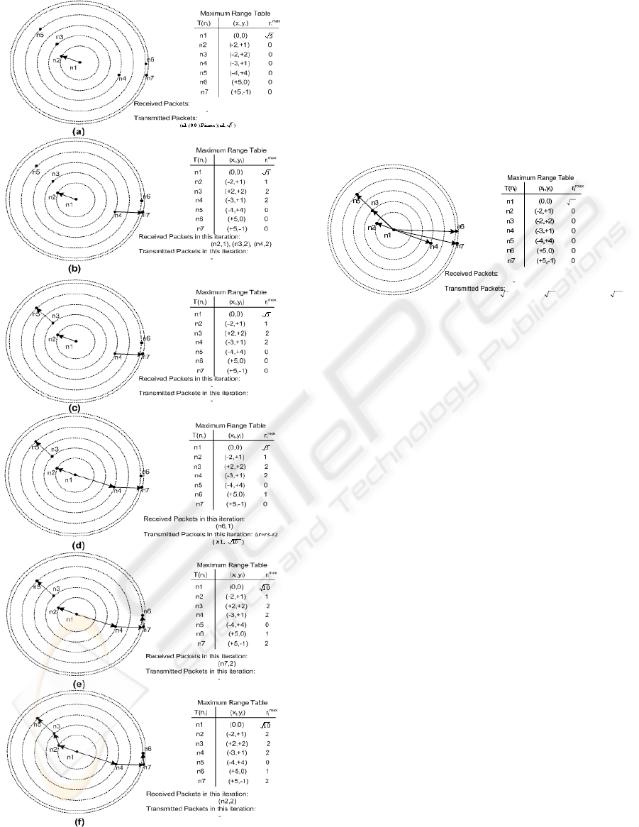
Figure 3: An example which illustrates running of ATC
algorithm for node
. (a) phase I and initialization step of
iteration 1 (b) Iteration 1 (c) Iteration 2 (d) Iteration 3 (e)
Iteration 4 (f) Iteration 5 of algorithm.
is recoverable and any one of them is not
retransmitted again. In a situation like this algorithm
1 works properly but the calculated maximum range
will not be the optimum value. Figure 4 shows the
result of algorithm 1 in the presence of 100% packet
loss.it should be mentioned that the assumed packet
loss is only for updates packets. In this situation the
maximum transmition range in our example will
change from
Figure 4: Result of the algorithm1 when node n
1
losses all
the received packets.
4 RESULTS AND DISCUSSION
In this section, we discuss the results of applying the
algorithm to a WSN and compare them with a
similar algorithm. In addition, the time and message
complexities of the proposed algorithm are
discussed.
A. Simulation Results
The efficiency of the proposed algorithm is
determined using some simulation results. We
compare the algorithm with a proposed scheme
against the algorithms given in (Liu and Li, 2003).
The algorithm has the most similarity to our work.
In this algorithm, Li and Liu present an asymmetric
algorithm based on Prim’s algorithm which is also a
distributed and local technique (Liu and Li, 2003).
Theoretically, (Liu and Li, 2003) calculates the best
local answer in our case. The efficiency of the
proposed algorithm is a function of the timer T
i
and
if we properly tune that, our approach could be as
efficient as (Liu and Li, 2003). In this study, we use
two schemes for the timer. In scheme I, we consider
the timer proportional to ∆
while in scheme II the
timer is assumed to be proportional to
.
Scheme I: Timer ~∆
Scheme II: Timer ~
The results are extracted using simulations in
MATLAB. The sensors, which are deployed in a
1000m 1000m area, are uniformly distributed. The
)26,1(),5,1(),4,1(),10,1(),2,1(),5(n1, nnnnn
26
ATC - An Asymmetric Topology Control Algorithm for Heterogeneous Wireless Sensor Networks
79
number of nodes is varied from 50 to 250. For every
data point, the simulation is repeated 10 times.
Table I shows the average node degree for the
topologies generated using the algorithms.
Theoretically, the best average node degree, denoted
by AND, is given by (Li et al., 2003)
AND =
∑
=
where n is the number of nodes. Note that
lim
2
The results show that the (Liu and Li, 2003) and
scheme II have the lowest AND. Fig. 4 compares the
average length of links (ALL) for the proposed and
(Liu and Li, 2003). As is evident from the figure, the
length decreases when the node density increases.
As the results show, the AND and ALL are about the
same for both the (Liu and Li, 2003) and our
proposed algorithm with scheme II. These
parameters are slightly more for the proposed
algorithm for sparse networks. For networks with
large scale scheme II operates as efficient as (Liu
and Li, 2003).
Table 2: Average node degree of the algorithms.
Algorithm
Proposed Algorithm
(Liu and
Li, 2003)
Scheme I Scheme II
Average
Degree
3.5 3 3
In figure 5, we compare the average power needed
to transmit 20 packets in the network between two
corners of our network position (0, 0) and (1000,
1000) under free space transmission model.
Comparison is between scheme I and II with LMST.
The results are normalized to results of LMST
method. As figure 5 shows the power result for
scheme II is quite near to LMST which has
minimum power among these classes of methods.
Scheme II consume slightly more power than
LMST.
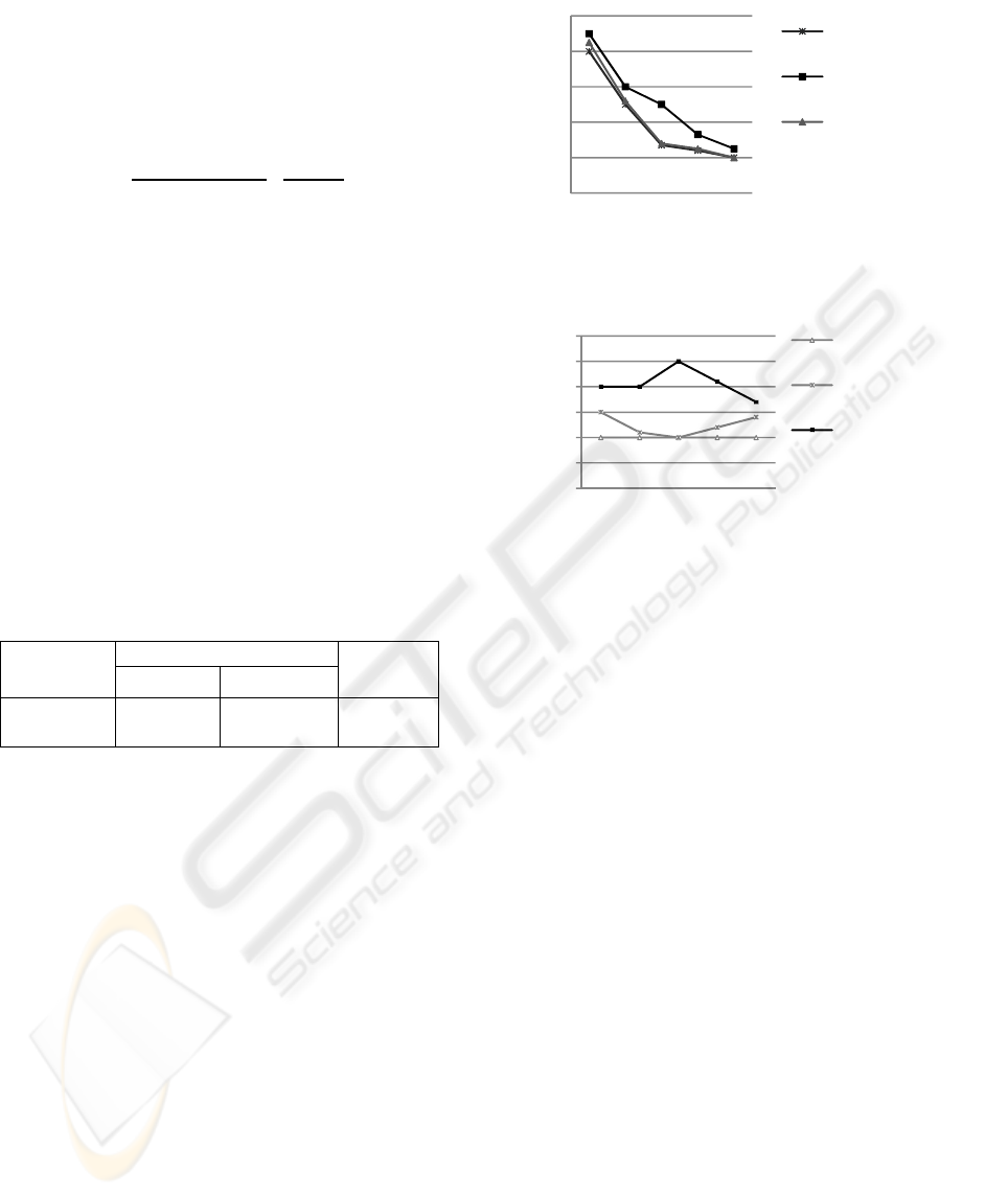
In figure 6, the results for the AND and ALL as a
function of update packet loss rate in phase II are
plotted. This figure shows the tolerability of the
algorithm against packet loss, while (Liu and Li,
2003) is quite sensitive to packet loss. The packet
loss rate ranges from 0% to 100% and the results are
for three network sizes of 50, 100, and 150 nodes.
As the results for the average node degree reveal, the
higher the packet loss rate is, the more ANDs we
will have. The algorithm operates at its best
efficiency when there is no packet loss. In this case,
Figure 4: Average length of links for different algorithms
as a function of the network size.
Figure 5: Power comparison of scheme I and scheme II
with LMST approach.
there are ANDs of 3.2, 3.3, and 3.5 for the network
sizes of 50, 75, 100, 125 and 150, respectively. The
differences between the ANDs of the networks
increase as the packet loss rate increases. The
performance of the proposed algorithm in an ideal
environment with no packet loss is almost as
efficient as the (Liu and Li, 2003). When the packet
loss increases, the efficiency of the algorithm
degrades. In the case of a 100% packet loss rate, the
algorithm performs like a primitive topology control
algorithm which adjusts the transmission power by
its farthest neighbor.
Figure 6(b) shows the variation of ALL when the
algorithm is applied to network with different sizes.
In situations where the low packet loss rate is low,
the algorithm works like LMST. The greater the
network size is, the smaller ALL will be. As the
packet loss rate increases, the algorithm works more
like the maximum topology control. In these cases,
the greater the network size is, the larger will be.
B. Algorithm Complexity
Time complexity: Let us denotes the number of
neighbors of
as Δ which is equal to
|
Ν
|
. The
number of algorithm iterations is Δ1. The
algorithm has Δ1 rounds. As a result, the time
complexity to construct
will be ΟΔ
. Also, in
each iteration, before the expiration of the timer T
i
,
40
60
80
100
120
140
50 100 150 200 250
AverageLinkLength(m)
Scheme[3]
Proposed
(SchemeI)
Proposed
(SchemeII)
0,9
0,95
1
1,05
1,1
1,15
1,2
50 100 150 200 250
NormalizedPower
NodeNumber
Scheme[3]
Proposed
(SchemeI)
Proposed
(SchemeII)
WINSYS 2010 - International Conference on Wireless Information Networks and Systems
80

at most Δ broadcast messages is received. This
makes the complexity of Algorithm1 equal to ΟΔ
.
Message Complexity: Assuming an ideal MAC
protocol with no collisions and retransmission, the
node
transmits at most
Δ1
1 messsages. A
hello message is transmitted at the beginning of the
protocol in the phase of the neighbor discovery and
at most Δ1 messages for updating the determined
levels of power
. Since each sensor has at most Δ
neighbors where each transmits ΟΔ messages, the
number of messages received by the sensor
is
ΟΔ
.
5 CONCLUSIONS
In this work, an Asymmetric Topology Control
(ATC) algorithm was proposed. In this algorithm all
the nodes simultaneously begin to transmission
range assignment and during transmission power
assignment, any modification in transmission range
will broadcast for all the neighbors.
Results show that algorithm works in a good
performance in comparison with similar algorithms
while preserve average node degree and average link
length. We also compare our algorithm to the LMST
algorithm which is a minimum power algorithm.
Results show our algorithm works as good as LMST
approach.
(a)
(b)
Figure 6: Performance evaluation for the proposed
algorithm versus the packet loss rate a) Average node
degree b) Average link length.
REFERENCES
S. Narayanaswamy, V. Kawadia, R. Sreenivas, and P.
Kumar, “Power control in ad hoc networks: Theory,
architecture, algorithm and implementation of the
COMPOW protocol,” in Proc. European Wireless
Conference – Next Generation Wireless Networks:
Technologies, Protocols, Services and Applications,
Florence, Italy, 2002, pp. 156–162.
V. Rodoplu, T. Meng, “Minimum energy mobile wireless
network,” IEEE journal selected Area in
Communications, vol. 17, pp.1333-1344, 1999.
J. Liu and B. Li, “Distributed Topology Control in
Wireless Sensor Networks with Asymmetric Links”,
in Proc. IEEE Glabal Telecommunication Conference,
2003, Vol. 3, pp. 1257- 1262.
N. Li, J. Hou, L. Sha, “Design and analysis of an mst-
based topology control algorithm,” in Proc. of the
IEEE Infocom 03, San Francisco, CA, 2003, pp. 1702-
1712.
L. Li, J. Y. Halpern, P. Bahl, and R. Wattenhofer,
“Analysis of a cone-based distributed topology control
algorithm for wireless multi-hop networks,” in Proc.
ACM Symposium on Principles of Distributed
Computing, 2001, pp. 264-273.
S. Narayanaswamy, V. Kawadia, R. Sreenivas and P.
Kumar, “Power control in ad hoc networks: Theory,
architecture, algorithm and implementation of the
COMPOW protocol,” in Proc. of European Wireless,
2002.
M. Cardei, S. Yang, J. Wu, “Algorithms for Fault-Tolerant
Topology in Heterogeneous Wireless Sensor
Networks,” IEEE Trans. on Parallel and Distributed
Systems, Vol 19, Issue 4, April 2008.
0
5
10
15
20
25
0
10
20
30
40
50
60
70
80
90
100
AverageDegree
Numberofnodes
50nodes
75nodes
100nodes
150nodes
125nodes
60
80
100
120
140
160
0 20406080100
AverageLinkLength(m)
Numberofnodes
50nodes
100nodes
150nodes
75nodes
125
ATC - An Asymmetric Topology Control Algorithm for Heterogeneous Wireless Sensor Networks
81
