
SPIDAR Calibration based on Neural Networks
versus Optical Tracking
Pierre Boudoin, Hichem Maaref, Samir Otmane and Malik Mallem
Laboratoire IBISC, Universit
´
e d’Evry, Evry, France
Abstract. This paper aims to present all the study done on the SPIDAR tracking
and haptic device, in order to improve accuracy on the given position. Firstly we
proposed a new semi-automatic initialization technique for this device using an
optical tracking system. We also propose an innovative way to perfom calibration
of 3D tracking device using virtual reality. Then, we used a two-layered feed-
forward neural network to reduce the location errors. We obtained very good
results with this calibration, since we reduced the mean error by more than 50%.
1 Introduction
Virtual reality is a domain which is highly dependent on tracking systems. Users in-
teract in 3 dimensions, with virtual entities in digital environments. In order to provide
the best user experience, it’s very important that 3D interaction has to be without any
interruption. This interaction relies on the transformation of a real movement into an
action in the virtual world. This work is done by a tracking solution. This tracking sys-
tem has to be reliable and the most available as possible. This point is crucial in order to
preserve data continuity and, so, data processing continuity and finally, 3D interaction
continuity. The main device used in our system is an optical tracking solution, it’s a
very accurate device. On the other hand, it suffers from a huge defect: tracking-loss.
That’s a particular true defect when only one marker is used. So, it’s essential to be
able to switch to another device in these situations in order to compensate this defect.
In our virtual reality system, we’ve got a SPIDAR [1] and we chose it to stand in for the
optical tracking system.
SPIDAR [1], for SPace Interaction Device for Augmented Reality, is an electrome-
chanical device, which has 8 couples of motor/encoder distributed on each vertex of a
cubic structure. A string is attached to each motor via a pulley. These 8 strings converges
to an effector. By winding their respective strings, each motor produces a tension. The
vectorial sum of these tensions produce the force feedback vector to be applied on the
effector, allowing the user to feel on what he is stumbling or to feel the weight of an ob-
ject. By observing the encoders values, the system can compute the 3D position of the
effector. The SPIDAR tracking is always available, but it suffers from a weak accuracy
and repeatability. So it’s impossible, when we want to 3D interact with accuracy, to use
raw position given by the SPIDAR without performing a calibration.
In our case, it’s a huge problem, since we used a 3D interaction technique, called
Fly Over [2], which needs a continuous position vector. This technique is based on
Boudoin P., Maaref H., Otmane S. and Mallem M. (2010).
SPIDAR Calibration based on Neural Networks versus Optical Tracking.
In Proceedings of the 6th International Workshop on Artificial Neural Networks and Intelligent Information Processing, pages 87-98
Copyright
c
SciTePress

different interaction areas offering to the user a continuity in the interaction. Indeed,
the least jump of position during the swing of a system, would be likely to pass the
pointer of Fly-Over of a zone of interaction towards another. This phenomenon involves
a behavior of the technique thus, not wished by the user and creating consequently a
rupture of the continuity of the 3D interaction. Thus, it’s important to propose measures
in order to consider the position given by the SPIDAR so that it is closest to the position
given by the optical tracking system, and so, minimizing effects on the 3D interaction.
This research work is presented as follow. First, we talk about similar works on
virtual reality devices calibration and correction. Then, we introduce our contribution
on a new SPIDAR calibration method using multimodal informations. After that, we
speak about the correction of the SPIDAR position using neural networks. Finally, we
discuss about a hybrid tracking system based on a SPIDAR and an optical tracking
solution.
2 Related Work
Since virtual reality systems use more and more devices, especially tracking devices,
it’s important to perform a good calibration of them. But not all tracking devices need
a huge correction, thus infrared based optical tracking devices are accurate enough and
so don’t need to be corrected. On the other hand, it exists some mechanical, electrome-
chanical or electromagnetic tracking devices which need to be calibrated and/or cor-
rected.
Most of research works has been realized on the electromagnetic tracking devices
because they suffers from electromagnetic distortions when magnetical materials are
placed into the tracking range. Moreover, the tracking accuracy falls off rapidly de-
pending on the distance from the emitter and the power of the emitter [3]. These effects
induce non-linear errors on the location. In order to correct them, it exists different
ways.
The easiest method is the linear interpolation [4] but it doesn’t correct non-linear
systems, so it’s very limited. Polynomial fitting [5, 6] allows to correct non-linear er-
rors. But depending on the number of coefficients, it could be very difficult using this
method in near realtime conditions because it will produce a heavy load for the system.
Moreover if the number of coefficient is too important, oscillations can appear, increas-
ing errors rather than decreasing them. Moreover, these techniques often fail to capture
small details in the correction. They are better in determining the overall shape of a
non-linear function. Kindratenko [7] and Saleh [8] worked on a neural network based
calibration of electromagnetic tracking systems and they obtained good results, better
than with other methods.
But all these techniques are based on interpolation and they need a valid set of data
to be effective. This set of data highly is often given by a calibration grid. A calibration
grid is a representation of a set of points. All these point have a known position and can
be compared with the position given by the device that we want to calibrate. But when
we’re working in 3D space, it’s very difficult to make use of it because it’s difficult to
place accurately a device on a 3D points. In order to realize that we can use another
88
mechanical device, such a robot arm or a haptic arm [9]. Or we can place accurately
passive sensors respecting a geometrical shape [10].
Our research work reaches these studies because the SPIDAR suffers from same
non-linear distortions and 3D calibration problematic. So, we search solutions in the
same direction.
3 Identification of the SPIDAR
3.1 Context
In order to preserve the data continuity, it is essential to correct a well-known prob-
lem appearing with tracking systems: data loss. Data loss appears when the tracking is
unable to update the position calculation, conducting to a jump in the data when the sys-
tem is re-enable to update the position. This phenomena is often mislead by occultation,
especially in optical tracking system. A data loss can be managed by three methods:
1. Prediction: We can predict the following data state by knowing the previous data
state through mathematical method , such Kalman filter.
2. Compensation: A device tracking loss, don’t forbid us to use another device. It’s
very important in this case that the data incoming from the different devices to be
expressed in the same space representation (same referential). This is necessary in
order to obtain a data continuity when the system switch from one device to another.
3. Correction: The last possibility is to correct data incoming from the most available
device, in our case the SPIDAR. To perform the correction, we could use the a priori
knowledge on the SPIDAR position through another device.
3.2 Design Problems
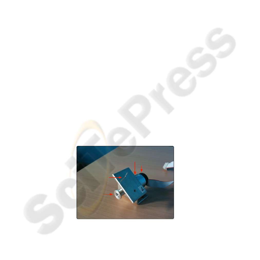
Guide
Pulley
Encoder
Motor
Fig. 1. Detailled view of a SPIDAR’s motor and its winding guide.
89
SPIDAR is an electromechanical device and consequently it could suffer from de-
sign problems more or less awkward for computing the effector’s position. These are
problems we have identified:
1. Encoders are Directly Mounted on the Motor’s Axis.
This is an important problem because we must define the pulley’s diameter in the
configuration file of the SPIDAR’s interface. However, this diameter is not constant,
depending on the quantity of string winded. So, this information is skewed.
2. Diameter of Pulleys is too Small.
The previous problem become more marked due to the small diameter of the pulley
used. Thus, the diameter being too small, it variates noticeably as strings being
winded go along. This phenomena would be less marked if the diameter used was
more important.
3. Winding Guides Badly Designed.
The present design of the winding guides, don’t prevent a string from missing the
pulley. This phenomena appears when the effector is being moved fast and con-
sequently, that motors have to wind an important quantity of string. This is a real
problem, because the encoder count one revolution but the string doesn’t be winded.
4. Size of Encoders. Encoders’ size is too small for counting the string quantity which
must be winded. When an encoder overflows, the counter is reseted and the winded
string quantity information is biased.
5. Dimensions of the SPIDAR. More dimensions are important and more every prob-
lem cited previously is marked. Some problems that are inconsiderable when di-
mensions are small, become not inconsiderable when dimensions are huge.
3.3 Experimental Protocol
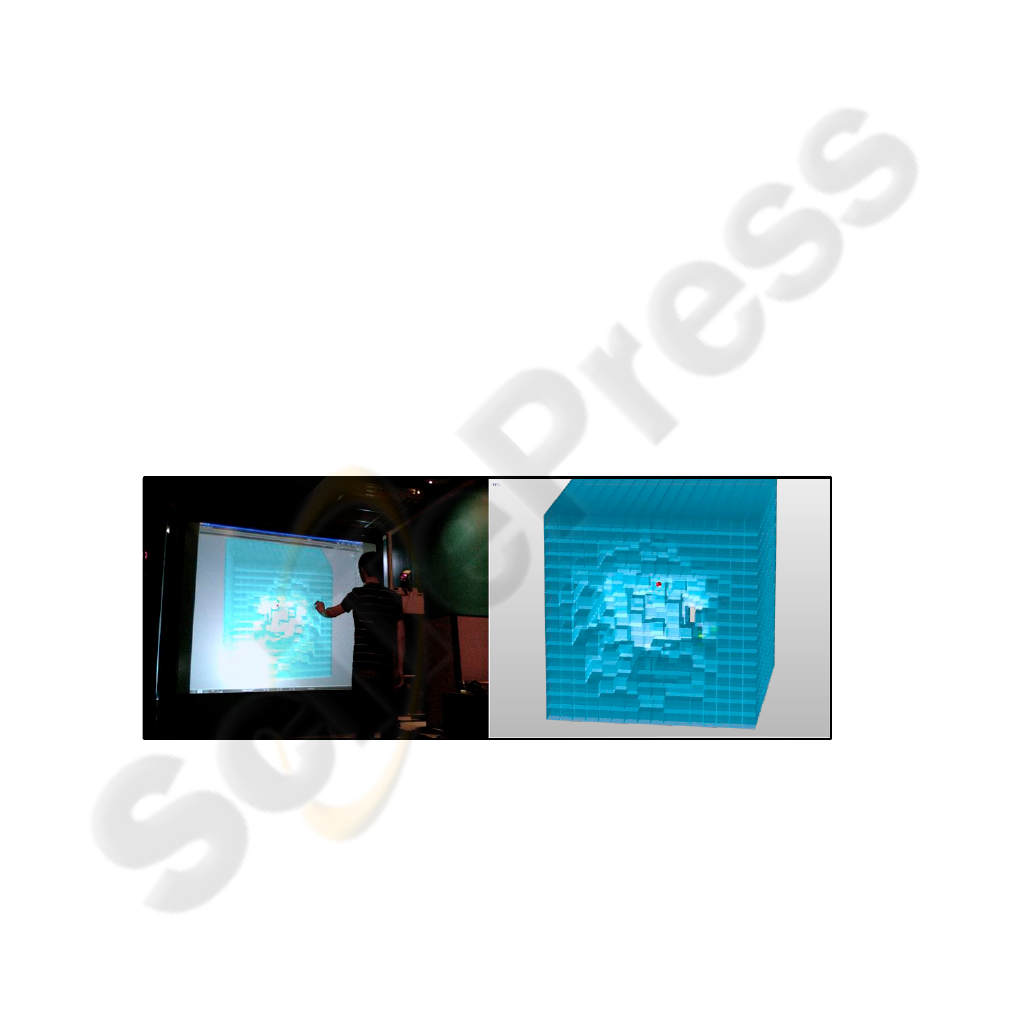
Fig. 2. On the left - A user using our virtual calibration grid in order to retrieve data for the neural
network learning. On the right - Detailed representation of the virtual calibration grid.
We use what we called: a virtual calibration grid (see fig.2), which consists in the rep-
resentation of a virtual scene, composed of many small cubes. Each cube corresponds
90
to a sub-space of the SPIDAR workspace. This set of small cubes covers the whole SP-
IDAR workspace. We recorded values, respecting this protocol in a workspace limited
to 1 m
3
split into 4096 sub-spaces (16 x 16 x 16). The great advantage of this protocol
is the homogeneity distribution of the data set.
The use of virtual reality for calibration allows more flexibility and less complexity
because we don’t have to move the SPIDAR effector with constraints or to place the
effector with a great accuracy on a set of calibration point.
This calibration grid, is represented Fig.2. We can identify the SPIDAR’s problem
with it, following these steps:
1. The user move the real effector (which is in his hand) in order to place the virtual
effector (which is a red sphere in the virtual scene) in each cube represented.
2. Each time the virtual effector is in collision with a cube, we record the position
given by the SPIDAR and the position given by the optical tracking.
3. Once these positions is recorded the cube disappears insuring that there will be only
one point for this sub-space.
3.4 Results
−500
0
500
−500
0
500
1000
1000
1200
1400
1600
1800
2000
X (mm)
Absolute error space distribution
Y (mm)
Z (mm)
0 mm
16 mm
31 mm
47 mm
62 mm
78 mm
93 mm
109 mm
124 mm
140 mm
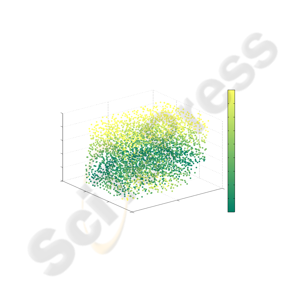
Fig. 3. Absolute error 3D distribution in the SPIDAR’s workspace (Dark green is the best).
Figure 3 represents errors’ space distribution. As we can see this is a onion skin dis-
tribution, meaning different spherical layers, the absolute error growing as the effector
is going in outside layers. This identification of the SPIDAR leads us to these observa-
tions:
91

- Firstly, the mechanical study tells us that too many design problems
- Moreover, it’s hard to quantify the final effect of these mechanical problems.
- Another problem, is the loss of knowledge towards the mathematical model used
by the SPIDAR to compute the effector’s position.
Finally, the SPIDAR suffers from a set of problems, which have more or less known
causes and for which we don’t know very well the influence on the whole system. In
order to enhance the SPIDAR’s accuracy, it could be interesting to orient ourself to
a solution capable of estimating/correcting the effector’s position without any knowl-
edge on the mathematical model. We choose to test that way using neural networks for
their capacities to learn a situation and to model any continuous mathematical function
without any information on the model.
4 Multimodal Initialization of SPIDAR
4.1 Context
The SPIDAR is a device which needs an initialization at each startup. Initialization
consists to define the origin of the referential in which 3D position will be expressed.
We realize this task by placing the SPIDAR’s effector in the center of its cubic structure
with the greatest accuracy. A worse initialization brings about a decline in accuracy
for the 3D position. Moreover, if the initialization is not identical at each startup, the
new referential won’t be the same and consequently prevent us from applying a data-
processing for correcting the SPIDAR’s position. So, it’s very important to realize this
initialization with a great attention. But, it’s very difficult to hand-place the effector in
the center of the SPIDAR structure with accuracy, due to the lack of markers to estimate
this.
4.2 Proposition
Our contribution brings a semi-automatic SPIDAR initialization. This initialization use
multi-modality in order to guide the user. These modalities are vision, audio and haptic.
In order to carry out the more accurate initialization, we need to determine the initial-
ization point in space with great accuracy. To realize that, our idea is to use the optical
tracking system we have on our VR platform (and in most common VR platform). This
tracking system offers a lower than 1 mm precision.
The geometrical disposition of IR cameras are known and the origin of the optical
tracking system too. We also know the theoretical initialization point of the SPIDAR.
Thus, we could determine the theoretical initialization point within the optical tracking
referential. In order to know the position of the effector in the optical tracking space, we
put an optical marker on it. Thus, if we compute the vector defined by the initialization
point and the position of the effector, we could get the distance from the initialization
point and the direction needed in order to converge to it.
92

s(x), the sigmoid function regulating the force applied to the effector.
s(x) = e
−10(kxk−0.5)
2
if x ∈ [−0.5; 0.5] (4)
∆, the unit vector defining the direction to the initialization point. It’s computed
from the normalization of vector
−→
V :
−→
∆ =
1
k
−→
V k
·
−→
V (5)
F
Max
, the maximum force to be applied on the effector.
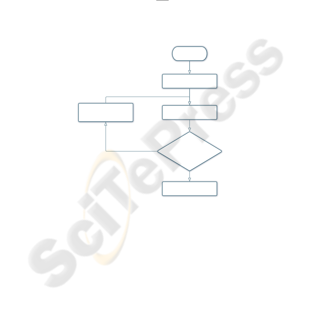
4.4 Initialization Algorithm
Start
SPIDAR initialization
Retrieving optical
tracking position
Optical tracking
position
= Calibration point
±�
Computing force to
converge to the
calibration point
No
Defining new referential
for SPIDAR
Yes
Fig. 5. SPIDAR initialization process algorithm.
Initialization process is done in two steps. A first initialization allows the user to
place the effector in a area near from the initialization point with a 1 or 2 cm accu-
racy. We can’t decrease below this distance using directly the SPIDAR’s force feedback
capabilities because it is not enough sensitive for moving the effector on small dis-
tances. In order to get a more accurate initialization, we need to add another step to the
initialization process. Using the different modalities previously cited, the user’s hand,
holding the effector, will be guided to converge to the initialization point with a 1.2 mm
accuracy.
94
5 Calibrating the SPIDAR with Neural Network
5.1 Configuration & Learning
We used a two-layered neural network, the first layer having a sigmoid activation func-
tion and the second a linear one. It’s a feed-forward back-propagation network using
the Levenberg-Marquardt learning algorithm [11]. The mean quadratic error is used as
performance function.
For the learning step, we use the SPIDAR’s position vectors in input and the optical
tracking’s position vectors in output because this is what we want in theory. However,
the whole vectors aren’t used, only data where the two tracking systems are available
has been used for the learning. It’s important for the learning step to remove data which
would decrease the neural network performances. Data income from the experimental
protocol described previously. So we obtain 4096 measure points. This data set has been
split into 3 sub-sets.
- 60% of data are used for the learning algorithm.
- 20% of data are used for the validation step, in order to prevent over-fitting phe-
nomenon.
- 20% of data are used to perform a generalization, that is the observation of the
neural network’s response to the introduction of set of totally unknown data (data
which haven’t be used for learning) in input.
5.2 Optimal Number of Neurons
4 6 8 10 12 14 16 18 20 22 24
12.5
13
13.5
14
14.5
15
15.5
16
16.5
Nombre de neurones VS erreur absolue moyenne en position
Nombre de neurones
Erreur absolue moyenne (mm)
4 6 8 10 12 14 16 18 20 22 24
12.5
13
13.5
14
14.5
15
15.5
16
16.5
Best
Number of neurons
Mean absolute learning error
Fig. 7. Mean absolute error versus number of neurons in the hidden layer.
The optimal number of neurons in the hidden layers has been defined in an empirical
way, by testing the result of learning with different number of neurons and by observ-
ing the mean absolute learning error. The more this error is high, the less the neural
network is effective. The figure 7 shows the mean absolute error on the SPIDAR posi-
tion according to the number of neurons in the hidden layer. By observing this result, we
could determine that the best configuration among the 3 to 21 neurons configurations,
is 5.
95


Table 2. Characteristic values of absolute errors on SPIDAR location in generalization with data
set 1.
Data set 1 Raw NN PF1
mean (mm) 13.23 5.31 7.91
std (mm) 8.41 5.14 7.68
max (mm) 37.60 29.42 32.51
6 Conclusions
In this paper we propose a method to calibrate SPIDAR using a feedforward neural
network coupled with a semi-automatic initialization. The semi-automatic initialization
allows us to place the SPIDAR referential at the same 3D position at each startup with an
accuracy of 1.2 mm. This way, we can use a method for calibrating the SPIDAR which,
don’t need to be updated at each startup. We choose a feedforward neural network
in order to compensate non linear errors on location and their abilities to estimate a
targeted output from a source without any knowledge on the mathematical model. We
obtain good results and our whole calibration procedure is efficient. Testing our neural
network in generalization shows us that our calibration is quite robust, even if we reset
the SPIDAR. We plan to make the initialization procedure fully automatic.
References
1. Kim, S., Ishii, M., Koike, Y., Sato, M.: Development of tension based haptic interface and
possibility of its application to virtual reality. Proceedings of the ACM symposium on Virtual
reality software and technology (2000) 199–205
2. Boudoin, P., Otmane, S., Mallem, M.: Fly over, a 3d interaction technique for navigation in
virtual environments independent from tracking devices. VRIC ’08 (2008) 7–13
3. Nixon, M., McCallum, B., Fright, W., Price, N.: The effects of metals and interfering fields
on electromagnetic trackers. Presence, 7, (1998) 204–218
4. Ghazisaedy, M., Adamczyk, D.: Ultrasonic calibration of a magnetic tracker in a virtual
reality space. Virtual Reality Annual International Symposium (VRAIS’95) (1995)
5. Bryson, S.: Measurement and calibration of static distortion of position data from 3d trackers.
Siggraph’92 (1992)
6. Ikits, M., Brederson, J., Hansen, C.D., Hollerbach, J.M.: An improved calibration framework
for electromagnetic tracking devices. IEEE Virtual Reality Conference 2001 (VR 2001)
(2001)
7. Kindratenko, V.: A survey of electromagnetic position tracker calibration techniques. Virtual
Reality,5, (2000) 169–182
8. Saleh, T., Kindratenko, V., Sherman, W.: On using neural networks to calibrate electro-
magnetic tracking systems. Proceedings of the IEEE virtual reality annual international
symposium (VRAIS ’95) (2000)
9. Ikits, M., Hansen, C., Johnson, C.: A comprehensive calibration and registration procedure
for the visual haptic workbench. Proceedings of the workshop on Virtual environments 2003,
39 (2003) 247–254
10. Leotta, D.: An efficient calibration method for freehand 3-d ultrasound imaging systems.
Ultrasound in medicine & biology (2004)
11. Bishop, C.: Neural networks for pattern recognition. Oxford University Press (2005)
98
