RELATIONSHIP BETWEEN LEVY DISTRIBUTION
AND TSALLIS DISTRIBUTION
Jyhjeng Deng
Industrial Engineering & Technology Management Department, DaYeh University, Chuang-Hua, Taiwan
Keywords: Mutator, Stable process.
Abstract: This paper describes the relationship between a stable process, the Levy distribution, and the Tsallis
distribution. These two distributions are often confused as different versions of each other, and are
commonly used as mutators in evolutionary algorithms. This study shows that they are usually different, but
are identical in special cases for both normal and Cauchy distributions. These two distributions can also be
related to each other. With proper equations for two different settings (with Levy’s kurtosis parameter
α
<
0.3490 and otherwise), the two distributions match well, particularly for
21
≤
≤
α
.
1 INTRODUCTION
Researchers have conducted many studies on
computational methods that are motivated by natural
evolution [1-6]. These methods can be divided into
three main groups: genetic algorithms (GAs),
evolutionary programming (EP), and evolutionary
strategies (ESs). All of these groups use various
mutation methods to intelligently search the
promising region in the solution domain. Based
upon these mutation methods, researchers often use
three types of mutation variate to produce random
mutation: Gaussian, Cauchy and Levy variates.
Gaussian and Cauchy variates are special cases of
the Levy process. Lee et al. (Lee and Yao, 2004)
introduced the Levy process, used Mantegna’s
algorithm (Mangetna, 1994) to produce the Levy
variate, and showed that the algorithm is useful for
Levy’s kurtosis parameter
0.7>
α
. Iwamatsu
generated the Levy variate of the Levy-type
distribution, which is just an approximation, using
the algorithm proposed by Tsallis and Stariolo
(Iwamatsu, 2002). Iwamatsu’s contribution is the
usage of Tsallis and Stariolo’s algorithm to generate
the Tsallis variate and apply it to the mutation in the
evolutionary programming. The Tsallis variate is not
the Levy stable process, but is very similar. The
paper first introduces the stable process and Tsallis
distribution. Equations show that these two
distributions are generally different, but are identical
for two special distributions, i.e. the normal and
Cauchy distributions. This section also provides two
equations to link the parameters in the Levy
distribution and Tsallis distribution so that they can
be approximated to each other. Various examples
show that they are quite similar, but not identical.
The Levy stable process can not only be used in
simulated annealing, evolutionary algorithms, as a
model for many types of physical and economic
systems, it also has quite amazing applications in
science and nature. In the case of animal foraging,
food search patterns can be quantitatively described
as resembling the Levy process. For example,
researchers have studied reindeer, wandering
albatrosses, and bumblebees and found that their
random walk resembles Levy flight behavior (see
example in Viswanathan et al. (Viswanathan and
Afanasyev, etal, 2000), Edwards et al. (Edwards and
Philips et al, 2007)). The strength of Levy flight in
animal foraging is obvious, as it helps foragers find
food and survive in severe environments.
2 THEORETICAL DEPLOYMENT
In probability theory, a Lévy skew alpha-stable
distribution or even just a stable distribution is a four
parameter family of continuous probability
distributions. The parameters are classified as
location and scale parameters μ and c, and two shape
parameters β and α, which roughly correspond to
measures of skewness and kurtosis, respectively.
The stable distribution has the important property of
stability. Except for possibly different shift and scale
360
Deng J. (2010).
RELATIONSHIP BETWEEN LEVY DISTRIBUTION AND TSALLIS DISTRIBUTION.
In Proceedings of the 12th International Conference on Enterprise Information Systems - Artificial Intelligence and Decision Support Systems, pages
360-367
DOI: 10.5220/0003002103600367
Copyright
c
 SciTePress

parameters, a stochastic variable, which is a linear
combination of several independent variables with
stable distribution, has the same stable distribution.
The Lévy skew stable probability distribution is
defined by the Fourier transform of its characteristic
function
(t)
ϕ
(Voit, 2003)
∫
∞
∞−
−
= )(
2
1
),,,;( dtetcxf
itx
ϕ
π
μβα (1)
where (t)
ϕ
is defined as:
()
(
)
Φ−−= )sgn(1exp(t) tictitu βϕ
α
(2)
where
)sgn(t
is just the sign of t, and Φ is given
by
(
)
2/tan
πα
=Φ
for all
α
except
α
= 1, in which case:
()
tlog/2 π −=Φ .
Note that the range of each parameter is the kurtosis
]2 ,0(∈
α
, the skewness
[] 1 ,1−∈
β
, the scale
0>c
, and the location
),( ∞−∞∈
μ
. Assuming
that the distribution is symmetric
()
0=
β
, the center
of its location is zero
()
0
=
μ
, then Eq. (2) can be
simplified as
(
)
α
ϕ ct-exp(t) =
. (3)
Inserting Eq. (3) into (1) produces
∫
∞
∞−
−
= )-exp(
2
1
)0,,0,;( dtectcxf
itx
α
π
α
. (4)
Let
α
γ c= (5)
and using the Euler formula
θθ
θ
sincos ie
i
+= (6)
and considering only the real part of Eq. (6), it is
easy to show that
∫
∞
==
0
,
)cos()t-exp(
1
)(L)0,,0,;( dttxxcxf
α
γα
γ
π
α
. (7)
This equation is identical to
)(L
,
y
γα
in Lee’s and
Mantegan’s paper, though the current study changes
the variable
y to x .
When
α
=2, the stable process in Eq. (3) becomes a
normal distribution. Using the characteristic function
of a normal distribution with a zero mean and a
variance of
2
1
σ
(Papoulis, 1990), which is
)
2
exp()(
22
1
t
t
σ
ϕ
−=
, it is easy to show that the variance
2
1
σ of Eq. (3) is
2
2c
. As for the Cauchy
distribution (
α
=1), its characteristics function is
)exp()( ctt −= ϕ
and the corresponding probability
density function is
2
2
)/(1
11
)(
cxc
xg
+
=
π
. (8)
The Tsallis distribution (Tsallis and Stariolo, 1996)
in one dimension is written as follows
)1/(1
)3/(2
2
)3/(1
2/1
)1(1
2
1
1
1
1
1
1
),;(
−
−
−−
⎭
⎬
⎫
⎩
⎨
⎧
−+
⎟
⎟
⎠
⎞
⎜
⎜
⎝
⎛
−
−
Γ
⎟
⎟
⎠
⎞
⎜
⎜
⎝
⎛
−
Γ
⎟
⎠
⎞
⎜
⎝
⎛
−
=
q
q
q
T
x
q
T
q
q
q
Tqxg
π
.(9)
Note that the ranges of parameters
q
and
T
are
)3,1[
∈
q
and
0>T
, respectively. The follow
section investigates the relationship between the
parameters
α
, c of
)0,,0,;( cxf
α
in Eq. (1) and
the
q and
T
of
),;( Tqxg
in Eq. (9).
According to Iwamatsu, when
+
→1q
, the Tsallis
distribution becomes a normal distribution
))/(exp(
1
),1;(
2
2
1
σ
πσ
xTqxg −=→
+
, (10)
and when q =2, it becomes the Cauchy distribution
2
2
)/(1
11
),2;(
σ
πσ
x
Txg
+
⋅=
. (11)
Note that
)3/(1 q
T
−
= σ
is a scale parameter, and is
not the usual meaning of standard deviation in a
RELATIONSHIP BETWEEN LEVY DISTRIBUTION AND TSALLIS DISTRIBUTION
361

normal distribution. The scale parameter
σ
is a
function of
q and
T
, and with different q it has
different function forms of
T
. For example, if
q =1, then
T= σ
, whereas if q =2, then
T
=
σ
.
The true standard deviation of the normal
distribution in Eq. (10) is
22
1
1
T
==
σσ
, which
renders the standard form of normal distribution as
))/(
2
1
exp(
2
1
),1;(
2
1
1
1
σ
πσ
xTqxg −=→
+
.(12)
As indicated above, the variance of normal
distribution as a special case of Levy distribution is
2
2c
and the variance of normal distribution as a
special case of Tsallis distribution is
2
T
. Therefore,
if the two normal distributions are identical, the
parameters between the Levy distribution and Tsallis
distribution must satisfy the following constraint,
2
2
2
T
c =
.
(13)
By the same token, apply the equality of the Cauchy
distribution and compare Eq. (8) and (11). It is clear
that
Tc
=
=
σ
. (14)
Equations (13) and (14) establish the link between
parameter
c of the Levy stable process in Eq. (7)
and the parameters
q and
T
of the Tsallis
distribution in Eq. (9) for the special cases of normal
(
α
=2,
q
=1) and Cauchy distributions (
α
=1,
q
=2).
Since this is derived only from special cases of
α
=1
or 2, this study proposes a general model between
parameters
c and
α
in Eq. (7) and parameters
q
and
T
in Eq. (9) as follows
)3/(1 q
Tc
−
= α . (15)
This model establishes the first relationship
between two sets of parameters
()
c ,
α
and
(
)
Tq ,
.
Note that when
α
=2 (which implies q =1), Eq.
(15) reduces to Eq. (13), whereas when
α
=1 (which
implies
q =2), Eq. (15) reduces to Eq. (14). The
second relationship between
()
γ
α
,
and
(
)
Tq,
is
inspired by Mantegna’s equation,
()
()
πα
α
α
/1
0
1,
Γ
=L
(16)
which describes the probability density in Eq. (7)
with scale parameter
c =1（implying
γ
=1, through
Eq. (5)）at
0
=
x . Recall that when 0=x , the
probability density for Tsallis distribution renders
)3/(1
2/1
2
1
1
1
1
1
1
)0(
q
q
T
q
q
q
xg
−−
⎟
⎟
⎠
⎞
⎜
⎜
⎝
⎛
−
−
Γ
⎟
⎟
⎠
⎞
⎜
⎜
⎝
⎛
−
Γ
⎟
⎠
⎞
⎜
⎝
⎛
−
==
π
. (17)
Combining Eq. (16) and (17) leads to
()
)3/(1
2/1
2
1
1
1
1
1
1/1
q
T
q
q
q
−−
⎟
⎟
⎠
⎞
⎜
⎜
⎝
⎛
−
−
Γ
⎟
⎟
⎠
⎞
⎜
⎜
⎝
⎛
−
Γ
⎟
⎠
⎞
⎜
⎝
⎛
−
=
Γ
ππα
α
. (18)
Equation (18) gives another constraint between
parameter
α
in Eq. (7) and parameters
q
and
T
in Eq. (9) when
γ
=1. Since this equation (18) is
derived from the special case of
γ
=1, this study
proposes a general model between parameters
α
and
γ
in Eq. (7) and parameters q and
T
in Eq.
(9) as follows
()
)3/(1
2/1
/1
2
1
1
1
1
1
1
)(
/1
q
T
q
q
q
−−
⎟
⎟
⎠
⎞
⎜
⎜
⎝
⎛
−
−
Γ
⎟
⎟
⎠
⎞
⎜
⎜
⎝
⎛
−
Γ
⎟
⎠
⎞
⎜
⎝
⎛
−
=
Γ
πγπα
α
α
. (19)
Note that when
γ
=1, Eq. (19) reduces to Eq. (18).
Therefore, by combining Eq. (5), (15) and (19) and
making some substitution in the parameters, this
study obtains two equations to define the
relationship between
(
)
γ
α
,
and
()
Tq,
as
()
⎟
⎟
⎠
⎞
⎜
⎜
⎝
⎛
−
−
Γ
⎟
⎟
⎠
⎞
⎜
⎜
⎝
⎛
−
Γ
⎟
⎠
⎞
⎜
⎝
⎛
−
=
Γ
=
−
2
1
1
1
1
1
1/1
2/1
)3/(1/1
q
q
q
T
q
ππ
α
αγ
α
. (20)
Substituting Eq. (5) into Eq. (20), the similar
relationship between
(
)
c,
α
and
()
Tq, leads to
()
⎟
⎟
⎠
⎞
⎜
⎜
⎝
⎛
−
−
Γ
⎟
⎟
⎠
⎞
⎜
⎜
⎝
⎛
−
Γ
⎟
⎠
⎞
⎜
⎝
⎛
−
=
Γ
=
−
2
1
1
1
1
1
1/1
2/1
)3/(1
q
q
q
Tc
q
ππ
α
α
. (21)
ICEIS 2010 - 12th International Conference on Enterprise Information Systems
362

Equation (21) states that two constraints are
required to establish the relationship between the
Levy stable process parameters
()
c,
α
and the
Tsallis distribution parameters
()
Tq,
so that the two
distributions will be equal in the special cases of two
categories. The first category includes the normal
and Cauchy distributions, in which the Levy and
Tsallis distributions are identical. In the second
category, the scale parameter
c =1, and the Levy
and Tsallis distributions coincide only at the peak of
the distribution. We do not know how close these
two distribution match in other regions of the variate
domain in the second category. To determine the
relationship between these two X, apply equation
(21) as follows. For the special case of normal
equation（for stable process
α
=2 and for Tsallis
distribution
+
→1q ） we obtain
ππ
11
2
2/1
=
= Tc
. (22)
The first constraint in Eq. (22) states that
2
2
2
T
c =
, which is exactly the same as Eq. (13). This
shows that the two distributions are equal in the
special case of a normal distribution. For the special
case of a Cauchy equation
（for stable process
α
=1
and for Tsallis distribution
q
=2）, Eq. (21) yields
ππ
11
=
=
T
c
. (23)
The first constraint in Eq. (23) equals Eq. (14),
which shows that the two distributions are identical
in the special case of a Cauchy distribution. As
above, Eq. (20) can be substituted for
α
=2 and 1 to
obtain the following equations
ππ
γ
11
2
2/12/1
=
= T
(24)
and
ππ
γ
11
=
=
T
. (25)
Equations (24) and (25) define the constraints
between
(
)
γ
α
,
and
(
)
Tq,
for normal and Cauchy
distributions. Next, this study verifies a normal
distribution case using a graph. Let
α
=2 and
8.0
=
c , and by Eq. (22) we have
2
4cT = =2.56. (26)
The probability density of Eq. (7) can be
calculated through numerical integration.
Fortunately, John Nolan has developed a program,
stable.exe, to perform the required calculations and
made it available on his website. Using the
stable.exe program from Nolan (Nolan, 1998) to
evaluate the probability density function (pdf) of
Eq., (7) with
α
=2 and
8.0=c
, this study
compares it with the Tsallis pdf of
+
→1q and
T
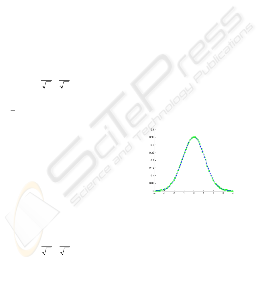
=2.56. Figure 1 shows the results of this graph
comparison, indicating that the pdfs are identical.
The blue line represents the stable.exe program and
the green squares represent the Tsallis pdf. This
study selects the
0
S
stable process in the stable.exe
and sets its gamma value at the
8.0=c
to calculate
its probability density function. In other words, the
gamma value in stable.exe is not
γ
but c in our
definition on the stable process in Eq. (1) and (5).
Figure 1: The comparison between Levy and Tasllis with
α
=2 and c =0.8.
This study also tests the Cauchy distribution with
α
=1 and c =0.75, and compares it with the Tsallis
pdf with
2
=
q
and
T
=0.75. Figure 2 shows these
results, which are clearly also identical.
RELATIONSHIP BETWEEN LEVY DISTRIBUTION AND TSALLIS DISTRIBUTION
363

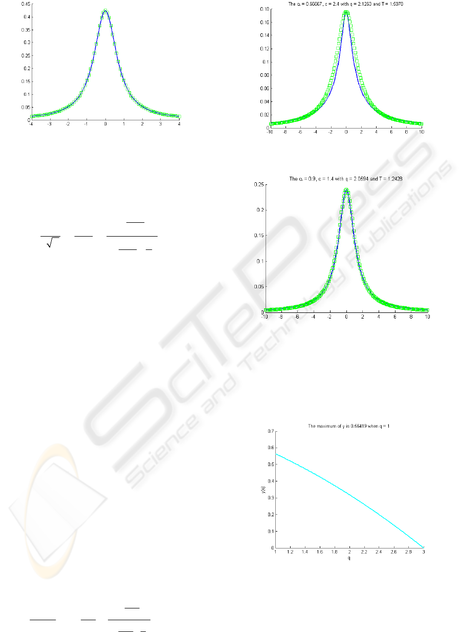
Figure 2: The comparison between Levy and Tasllis with
α
=1 and c =0.75.
Comparing the general cases of
α
=2/3 and c =2.4
and substituting them into Eq. (21) leads to
1/(3 )
1/2
1.6
1
1
11
211
12
q
T
q
q
q
π
π
−
=
⎛⎞
Γ
⎜⎟
−
−
⎛⎞
⎝⎠
=
⎜⎟
⎛⎞
⎝⎠
Γ−
⎜⎟
−
⎝⎠
. (27)
The right hand side of the second constraint in Eq.
(27) is clearly a monotonically decreasing function
of
q . Thus, the solution for q is uniquely
determined. Solving
q first in the lower part of Eq.
(27) produces
q
=2.1263. Substituting this value
into the upper part of Eq. (27) then leads to
T
=1.5078. Figure 3 compares the Levy distribution
with parameters
α
=2/3 and
c
=2.4 and the Tsallis
distribution with
q
=2.1263 and
T
=1.5078,
showing that they are not identical. This is not a
surprise because the Tsallis distribution is generally
not a Levy stable process, and Levy stable processes
usually do not have an analytical form except for
special cases [7]. However, they are quite close. This
means that the Tsallis distribution can be a good
approximation of the Levy distribution. Using the
values
α
=0.9 and c =1.4 produces similar results,
and Figure 4 shows that they are almost identical.
A comparison of Figures 3 and 4 clearly shows
that as
α
becomes smaller, the match between
Levy and Tsallis decreases. Equation (21) helps
explain the deviation between these two
distributions. For the sake of clarity, repeat the
second part of Eq. (21) in Eq. (28) as follows. Here
y
has two meanings: one is the function of
q
(
)(qy
); the other is the function of
α
()
)(
α
y
.
()
1/2
1
1/
1
1
11
12
q
q
y
q
α
ππ
⎛⎞
Γ
⎜⎟
Γ
−
−
⎛⎞
⎝⎠
==
⎜⎟
⎛⎞
⎝⎠
Γ−
⎜⎟
−
⎝⎠
(28)
Figure 3: The comparison between Levy and Tasllis with
α
=2/3 and c =2.4.
Figure 4: The comparison between Levy and Tasllis with
α
=0.9 and c =1.4.
As mentioned above, the right hand side of the
second equation in Eq. (21) is a monotonically
decreasing function of
q
for
]3,1(∈q
. Figure 5
shows the results.
Figure 5: Function of
)y(q
.
The maximum of
y
is 0.56419 when
+
→1q .
Note also that the left hand side of Eq. (28) is a
convex function of
α
. As
+
→ 0 α , )(
α
y
approaches to infinity and decreases to a minimum
ICEIS 2010 - 12th International Conference on Enterprise Information Systems
364

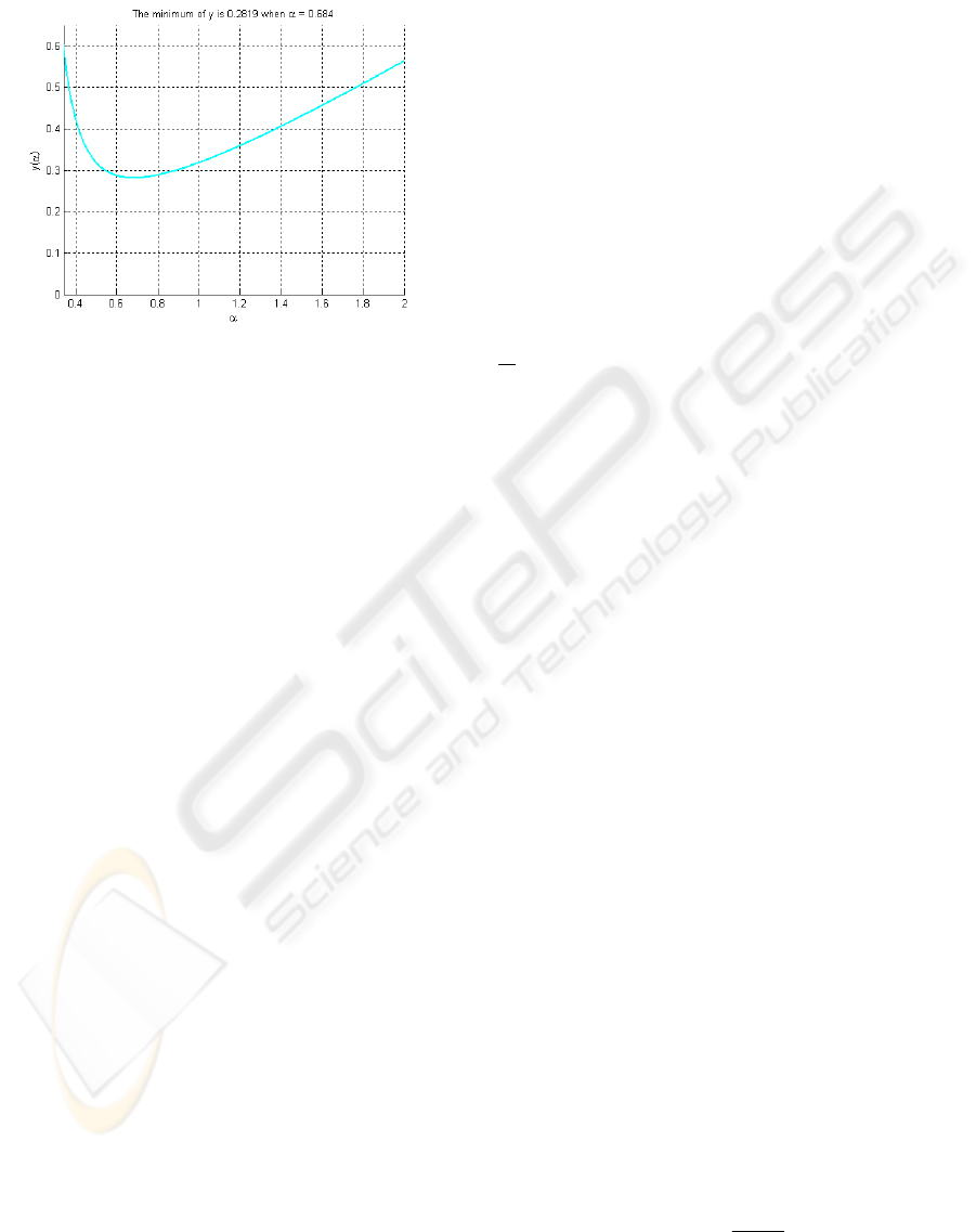
as
α
increases up to 0.684. Then )(
α
y climbs
upwards and reaches its local extreme when
α
goes
to 2. Figure 6 shows the results.
Figure 6: Function of
)(
α
y
.
To produce a solution of q for a given
α
in Eq.
(28), the value of )(qy in Fig. 5 must equal that of
)(
α
y in Fig. 6. Since the range of )(qy is less
than or equal to 0.56419 and the range of
)(
α
y can
go up to infinity, it is clear that for certain ranges of
α
, there is no solution for q that satisfies Eq. (28).
This creates the first problem. On the other hand,
since
)(
α
y is a convex function with a minimum
of 0.2819, thus for
)(qy
less than 0.2819 （which
implies that
>q
2.127）, there is no solution for
α
that satisfies Eq. (28). The third problem is related to
the second problem. When
[
]
( ) 0.2819,0.56419yq∈
,
there are two solutions for
α
. This creates the
possible dilemma that for a set of
()
Tq,
, there are two
sets of
()
c,
α
that satisfy Eq. (28). This means there is
a possibility that
()
Tq,
and
()
c, α
do not form a one-
on-one mapping, which is an undesirable situation.
The following section solves the third problem of
finding proper
()
c, α
given a set of
()
Tq,
. The other
two problems, are solved in a similar manner.
Two examples can be used to demonstrate the
procedure of solving two solutions for
α
. The map
between
()
c,
α
and
()
Tq,
can be unique even if there
are two solutions of
α
for a given q in Eq. (28).
Fix one
α
(where
α
<0.684) first, and then use Eq.
(28) to determine its left hand side. Then solve
another
α
(where
α
>0.684) by applying the left
hand side of Eq. (28) again. This approach produces
two values of
α
(say,
1
α
and
2
α
) for a common
)(
α
y
. Using the right hand side of Eq. (28), solve
for a unique
q . Further, assume a value of
T
such
that there are two sets of
(
)
c,
α
, say
()
11
, c
α
and
(
)
22
, c
α
, in Eq. (21) for a given set of
(
)
Tq,
.
Which one of
(
)
11
, c
α
and
()
22
, c
α
is a better
match to
(
)
Tq,
? Numerical examples show that a
significant difference may exist between
()
11
, c
α
and
(
)
22
, c
α
in the matter of resemblance to
(
)
Tq,
.
Thus, find two sets of
(
)
c,
α
, which are
()
11
, c
α
and
(
)
22
, c
α
, and compare them to the
()
Tq,
to find
a better match between
()
c, α
and
()
Tq,
. The
following section provides two numerical examples.
First let the first choice of
α
(where
α
>0.684) be
1
α
=1, then the left hand side of Eq. (28) is
1
0.3183
π
=
, and the other
α
(where
α
<0.684),
which renders the same
)(
α
y , be
2
α
=0.5. In both
cases, the corresponding
q =2. Now further assume
that
T
=1, and substitute
α
=
1
α
=1,
T
=1, and
q =2 into the upper part of Eq. (21). This produces
c =
1
c
=1, which is a standard Cauchy distribution,
and is the same result obtained above. The Levy
distribution (with parameters
1
α
=1 and
1
c
=1) and
Tsallis distribution (with parameters
q =2 and
T
=1) coincide. On the other hand, substituting
α
=
2
α
=0.5,
q
=2, and
T
=1 leads to c =
2
c =2. It
is clear that the Levy distribution (with parameters
2
α
=0.5 and
2
c =2) is not a Cauchy distribution, and
therefore will not be equal to the Tsallis distribution
(with parameters
q =2 and
T
=1). Figure 7 shows
the departure between
α
=0.5,
c
=2, and q =2,
T
=1. This figure shows that the departure can be
quite large between
(
)
c,
α
and
()
Tq,
for an
improper choice of
(
)
c,
α
. Thus, selecting the
correct values of
(
)
c,
α
for a given value of
(
)
Tq,
is a crucial task: the right choice leads to an exact
match, whereas the wrong choice produces an out of
shape match.
Next, consider the first problem: how to find
q
when
α
< 0.3490? The solution in this study is
based on Deng’s paper [22], in which the
relationship between
α
and
q
when ∞→
x
is
α +
+=
1
2
1q
. (29)
RELATIONSHIP BETWEEN LEVY DISTRIBUTION AND TSALLIS DISTRIBUTION
365

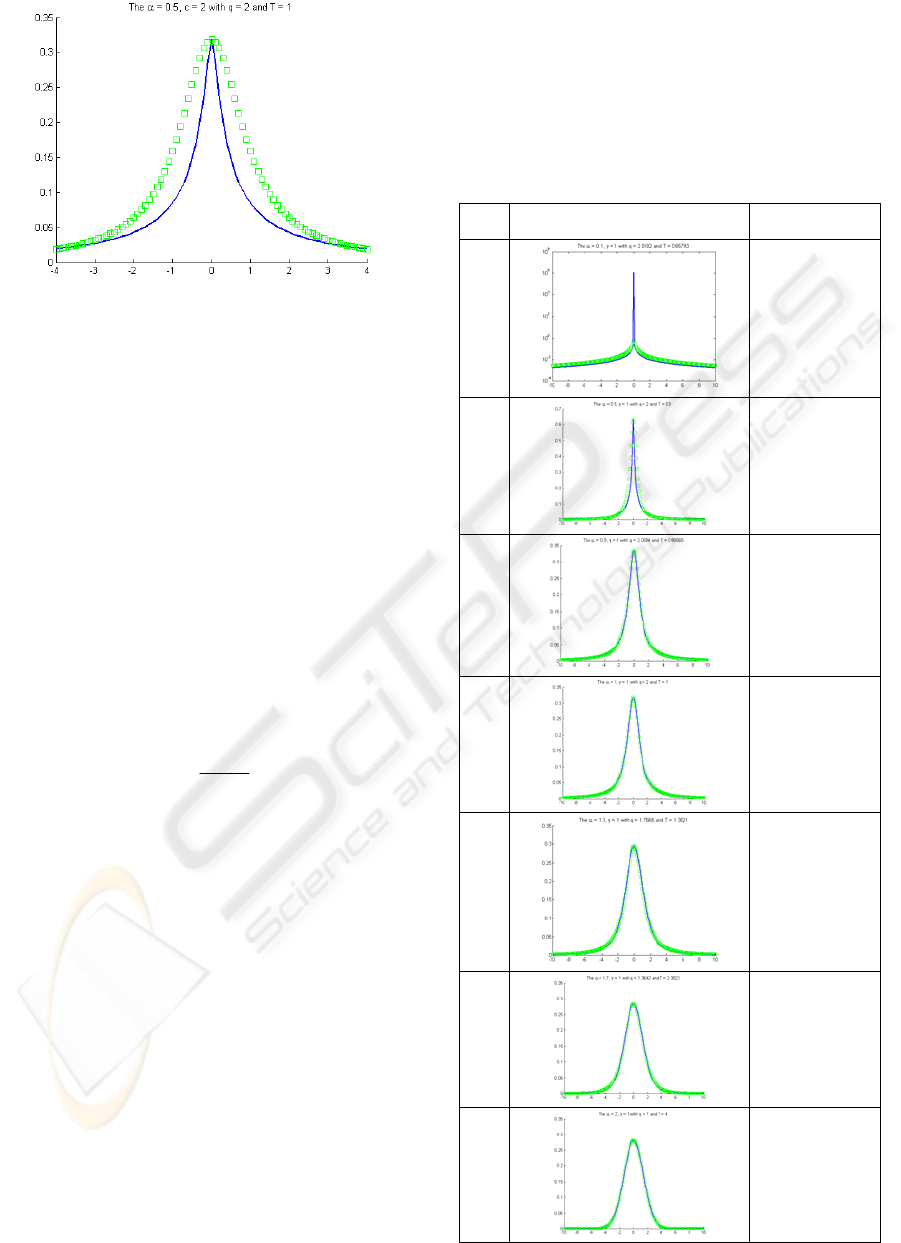
Figure 7: The comparison between
α
=0.5,
c
=2 (blue
line), and
q
=2,
T
=1 (green squares).
Equation (29) clearly shows that as
+
→ 0 α
,
−
→ 3q
. Recall that the range for
α
is ]2,0( and
the range for q is )3,1[ . Therefore, Eq. (29)
satisfies the one to one relationship between
α
and
q when
α
< 0.3490. Note that Eq. (29) also solves
the second problem, i.e., when
q > 2.127 there is no
solution of
α
in Eq. (28). Simply replacing Eq. (28)
with Eq. (29) immediately solves the first and
second problems. Combining Eq. (29) with the first
part of Eq. (21) produces a new equation for solving
()
Tq, given a set value of
()
c,
α
when
α
<
0.3490. This equation is
α
α
+
+=
=
−
1
2
1
)3/(1
q
Tc
q
. (30)
The purpose for substituting Eq. (29) for Eq. (28) is
to focus on the match between the two distributions
in the heavy tails instead of on the peak of the
distribution. This is because the heavy tails count
more (or have more impact) when
α
< 0.3490. To
show the effect of Eq. (21) and (30), try different
α
values with
=c
γ
=1 using Eq. (21) and (30).
Check the relationship between
α
and the match
quality between the two distributions. Table 1 lists
these results, showing that when
1≥
α
, the match
quality between Levy and Tsallis distributions is
either perfect or excellent. At
1<
α
, the quality
deteriorates a bit. When
α
< 0.3490, the two
distributions match very well on the heavy tails
except for the narrow region near the origin, where
they are significantly different. Note that the blue
line represents the Levy stable process, whereas the
green squares stand for the Tsallis distribution. Note
that for the case of
α
=0.1, the green squares rise
above the blue line in the region from
1010
≤
≤
−
x . If the domain of
x
is extended in
absolute value to 10000, the two will match almost
exactly on the heavy tails. This result is not shown
here for the sake of brevity. The difference between
Table 1: Match quality vs various
α
.
α
Graph result Match quality
0.1
fair
0.5
good
0.9
good
1.0
exact
1.3
excellent
1.7
excellent
2.0
exact
ICEIS 2010 - 12th International Conference on Enterprise Information Systems
366

them is less than
7
10*5.1
−
in absolute value. Taking
the Levy stable process as the standard and
approximating it by the Tsallis distribution shows
that the relative deviation is about 11.35%. The
relative deviation decreases as the absolute value of
x
increases.
3 CONCLUSIONS
This study thoroughly investigates the relationship
between the parameters
(
)
c,
α
and
()
Tq,
in the
Levy distribution and the Tsallis distribution.
Results show that they are usually totally different,
except for two special cases of normal and Cauchy
distributions. However, they can be approximated to
each other through linking equation in (21) or (30)
depending on whether or not the kurtosis parameter
is
α
< 0.3490. When 1≥
α
, the match quality
between the Levy and Tsallis distributions is either
perfect or excellent. When
α
<1, the quality
deteriorates a bit. When
α
<0.3490, except on the
narrow region near origin where the two have a
significant difference, the two match very well on
the heavy tails.
ACKNOWLEDGEMENTS
The author wish to give thanks for the grant from
NSC in Taiwan with contract NSC-98-2221-E212-
018-MY2.
REFERENCES
Edwards, A.M., Philips, R.A. Watkins, N.W., et al, 2007.
Revisiting Levy Flight Search Patterns of Wandering
Albatrosses, Bumblebees, and Deer, Nature 449 pp.
1044-1049.
Iwamatsu, M., 2002, Generalized evolutionary
programming with Levy-type mutation, Computer
Physics Communication 147, pp. 729-734.
Lee, C.-Y. and Yao, X., 2004. Evolutionary programming
using mutations based on the Levy probability
distribution, IEEE Transactions on Evolutionary
Computation, pp. 1-14.
Nolan, J.P., 1998. Parametrizations and modes of stable
distributions, Stats. & Proba. Letters, 38 pp. 187-195.
Papoulis, A., 1990. Probability & Statistics, Prentice Hall,
NJ.
Viswanathan, G.M., Afanasyev, V., Buldyrev, S.V., et al,
2000. Levy Flights in Random Searches, Physica A
282 pp 1-8.
Voit, J., 2003 The Statistical Mechanics of Financial
Markets (Texts and Monographs in Physics), Springer-
Verlag, Berlin.
RELATIONSHIP BETWEEN LEVY DISTRIBUTION AND TSALLIS DISTRIBUTION
367