INFERENCE OF BRAIN MENTAL STATES FROM

SPATIO-TEMPORAL ANALYSIS OF EEG SINGLE TRIALS

Yehudit Hasson-Meir, Andrey Zhdanov

The Balvatnik School of Computer Science, Tel-Aviv University, Tel-Aviv, Israel

Talma Hendler

, Nathan Intrator

The Functional Brain Imaging Unit, Wohl Institute for Advanced Imaging, Tel Aviv Sourasky Medical Center, Israel

The Balvatnik School of Computer Science, Tel-Aviv University, Tel-Aviv, Israel

Keywords: EEG, Brain computer interface, Regularization, Spatio-temporal analysis.

Abstract: We present an efficient and robust computational model for brain state interpretation from EEG single trials.

This includes identification of the most relevant time points and electrodes that may be active and contribute

to differentiation between the mental states investigated during the experiment. The model includes a

regularized logistic regression classifier trained with cross-validation to find the optimal model and its

regularization parameter. The proposed framework is generic and can be applied to different classification

tasks. In this study we applied it to a classical visual task of distinction between faces and houses. The

results show that the obtained single trial prediction is significantly better than chance. Moreover, correct

choice of the regularization parameter significantly improves classification results. In addition, the obtained

spatial-temporal information of brain activity can give an indication to correlated activity of regions of the

brain (spatial) as well as temporal activity correlations between and within EEG electrodes. This spatial-

temporal analysis can render a far more holistic interpretability for visual perception mechanism without

any a priori bias on certain time periods or scalp locations.

1 INTRODUCTION

A major challenge in neuroscience is inferring how

momentary mental states are mapped into a

particular pattern of brain activity. Inference, which

is based on EEG single-trial (i.e. short segment of

the EEG) has practical implementations for brain

computer interface (BCI) applications. Those BCI

applications are designated for people suffering from

physical disabilities, by helping them to

communicate with an electronic device through

decoding their brain signals in real time (Wolpaw

et al., 2002; Allison et al., 2007; Dornhege et al.,

2007; Blankertz et al., 2007).

The most common way to analyze EEG single-

trials is through classification (for review, see Lotte

et al., 2007). One of the main challenges of

classifying EEG single-trial signals is the amount of

data needed to properly describe the different states.

The later increases exponentially with the

dimensionality of the data; this is known as the curse

of dimensionality problem (Bellman, 1961).

To reduce the dimension of the data, many feature

selection methods have been developed for

identifying and choosing an optimal subset of

features from the data. Often, researchers focus on

few electrodes based on algorithms for channel

selection, which pick the most promising channels

for classification. Muller et al. (2000) utilized

Spatial Pattern Analysis and PCA for channel

selection and compared it to a set of four electrodes

chosen based on prior knowledge.

As a result,

Spatial pattern analysis enhanced the higher

classification rate; (Palaniappan et al., 2002) and

(Schröder et al., 2003) found the appropriate

channels via a Genetic Algorithm; (Lal et al., 2004)

used Recursive Feature Elimination and Zero-Norm

Optimization to reduce the number of electrodes

from 39 to 12. (Tomika and Muller, 2010) reduced

the dimension of the data by down-sampling the

signals.

Hasson-Meir Y., Zhdanov A., Hendler T. and Intrator N..

INFERENCE OF BRAIN MENTAL STATES FROM SPATIO-TEMPORAL ANALYSIS OF EEG SINGLE TRIALS.

DOI: 10.5220/0003159800590066

In Proceedings of the International Conference on Bio-inspired Systems and Signal Processing (BIOSIGNALS-2011), pages 59-66

ISBN: 978-989-8425-35-5

 2011 SCITEPRESS (Science and Technology Publications, Lda.)

Another way to alleviate the curse of

dimensionality is via regularization methods, which

stabilize the solutions by introducing prior

knowledge or by restricting the solution (Jain et al.,

2000; Duda et al., 2001). Cross-validation can be

used to find the optimized model and its

regularization parameter (Tomioka and Muller,

2010; Christoforou et al., 2008; Tomioka et al.,

2007; Zhdanov et al., 2007).

As data is becoming more readily available, it is

more desirable to let the data guide the choice of the

model (namely, determine the most relevant

electrodes and most relevant time points) while

minimizing a-priori assumptions. Therefore, a two-

dimensional representation of the spatio-temporal

predictive information of the brain activity is highly

needed for research and diagnosis, especially for

development of new paradigms, for which the neural

correlates may not be known in advance (Murray et

al., 2008).

Modern data-driven analyses, such as microstate

segmentation (Lehmann and Skrandies

, 1980;

Lehmann et al., 1987), have been developed and

used to study the spatio-temporal activity in the

brain. Microstate segmentation uses the spatial

distribution of the ERP which involves averaging

over multiple trials of similar brain activity (for

review, see Murray et al., 2008). Such a predictive

map lacks the correlated activity between electrodes.

This correlation information is lost in the traditional

ERP approach. Moreover, the ability to assess the

trial-to-trial variability in event-related potential

experiments can provide new insights into brain

function which may be ignored during ERP

averaging.

(Tomioka and Muller, 2010) suggested an EEG

single trials spatio-temporal interpretation, which

was based on three different regularizers. The

regularizers were used to reveal different and

complementary aspects of the localization of the

discriminative information. (The channel selection

regularizer was used for spatially localizing the

discriminative information, the temporal-basis

selection regularizer localized the discriminative

information in the temporal domain and the DS

regularizer provided a small number of pairs of

spatial and temporal filters that showed both spatial

and temporal localization of the discriminative

information in a compact manner). The regularizers

were applied on a block diagonal data matrix

concatenated first order changes (short segment of

filtered EEG signal with C channels and T sampled

time-points) and second order changes (the

covariance matrix of a short segment of band-pass

filtered EEG). The proposed model has shown

competitive performance against conventional

methods.

However, the deriving complexity of the learning

problem is high due to the size of the data matrix.

Moreover, using down sampling for reducing the

data dimension does not solve the problem, as it

ignores important properties of the signal, which are

visible in the EEG high temporal resolution. The use

of different regularizers (Tomioka and Muller, 2010)

may be problematic as it may produce contrasting

interpretations with no clear ability to determine

which of them is more accurate.

In this work, we follow the framework introduced

by (Zhdanov et al., 2007) and present an efficient

and robust computational model for brain state

interpretation from EEG single trials. Our approach

is based on the use of regularization techniques to

optimize the classifier coefficients and find the

correct model. We further demonstrate how to

identify the most relevant time points and electrodes

that might be most pertinent in contributing to

differentiation between the mental states

investigated.

Our approach employs a two-step classification:

First we locate the most informative time points and

the most active electrodes in these time points. Then

we try to combine some time points together to

analyze the information flow in the brain related to

the paradigm. This two-step framework allows us to

use a small number of parameters (dozens of

parameters compared with thousands parameters in

(Tomioka and Muller, 2010)) and maintain a high

temporal resolution of the EEG data. In addition, our

spatio-temporal analysis of the brain activity is

presented in one model, which makes it clear and

easy to interpret.

The proposed framework is generic and can be

applied to different classification tasks. In this study

we applied it to a classical visual task of distinction

between faces and houses.

2 MATERIALS AND METHODS

2.1 Experiment Setup

Four subjects (SUBJ1-SUBJ4, 4 females, two left

handed, aged 23-28), participated in this experiment.

All subjects gave informed consent to participate in

the study, which was approved by the ethics

committee of the Tel Aviv Sourasky Medical

Center. Subjects were presented with images from

two different categories-faces and houses. The

BIOSIGNALS 2011 - International Conference on Bio-inspired Systems and Signal Processing

images of faces were taken from the (Ekman and

Friesen, 1976) and (Lundqvist et al., 1998) databases

and include fearful or neutral facial expression.

The experiment included 4 sessions, each of 138

epochs 2- seconds-long. During each epoch, the

subject was presented with one image of a fearful

face, neutral face, house or blank (32, 32, 64 and 10

epochs respectively). To achieve visual field

segregation, participants were explicitly instructed to

ignore the pictures and to concentrate on a fixation

dot at the center of the screen. Throughout the

experiment, participants were asked to report the

color change of the central fixation dot.

2.2 EEG Data Acquisition

Continuous EEG data was recorded simultaneously

with fMRI acquisition. In this study, we are focusing

on the EEG data and have set aside the combined

fMRI data for further research. Good signal-to-noise

ratio of the EEG data in the combined approach was

previously shown at our lab (Sadeh et al., 2008;

Ben-Simon et al., 2008).

We used a 32-channel BrainCap electrode cap

with

sintered Ag/AgCl ring electrodes (30 EEG

channels, 1 ECG channel and 1 EOG cannel, Falk

Minow Services, Herrsching-Breitbrunn, Germany)

and a MR-compatible, 32-channel, battery-operated

amplifier (Brain Products, GmBH, Germany). The

electrodes were positioned according to the 10/20

system. The reference electrode was between Fz and

Cz (

Laufs et at., 2003). The signal was amplified,

and sampled at 5000 Hz using the Brain Vision

Recorder software (Brain Products). The EEG data

was transmitted from the scanner room via an

optical fiber to a PC in the control room. The exact

timing of stimulus onset and MRI scanner gradient

switching was transmitted to the EEG amplifier and

recorded together with the EEG signal.

2.3 EEG Analysis

EEG analysis were performed with EEGLAB 6.01

software package (Schwartz Center for

Computational Neuroscience, University of

California, San Diego), MATLAB software and

FMRIB plug-in for EEGLAB, provided by the

University of Oxford Centre for Functional MRI of

the Brain (FMRIB). Pre-processing of the EEG data

included the following steps: MR gradient artifacts

removal and Cardio-ballistic artifacts removal using

a FASTR algorithm implemented in FMRIB plug-in

for EEGLAB (Sadeh et al., 2008; Ben-Simon et al.,

2008).

For computational efficiency, the EEG signals

were down-sampled to 250 Hz and eye blinking

artifacts were removed using ICA (Delorme et al.,

2001). The data was then filtered with a 0.5–45 Hz

band-pass filter and segmented into epochs starting

100 ms before the stimulus onset and ending 600

after the stimulus onset. Baseline correction was

performed using the 100ms of pre-stimulus activity.

In this manner for each subject, we obtained

several dozens of epochs, each containing 32

(number of channels) x 175 (number of time

sampling points in the segmented interval) values.

Each epoch was associated with a class label "face"

or "house" according to the stimulus which was

presented.

3 BRAIN STATE MODELLING

In this section, we introduce the proposed brain state

modelling approach for EEG single trials spatio-

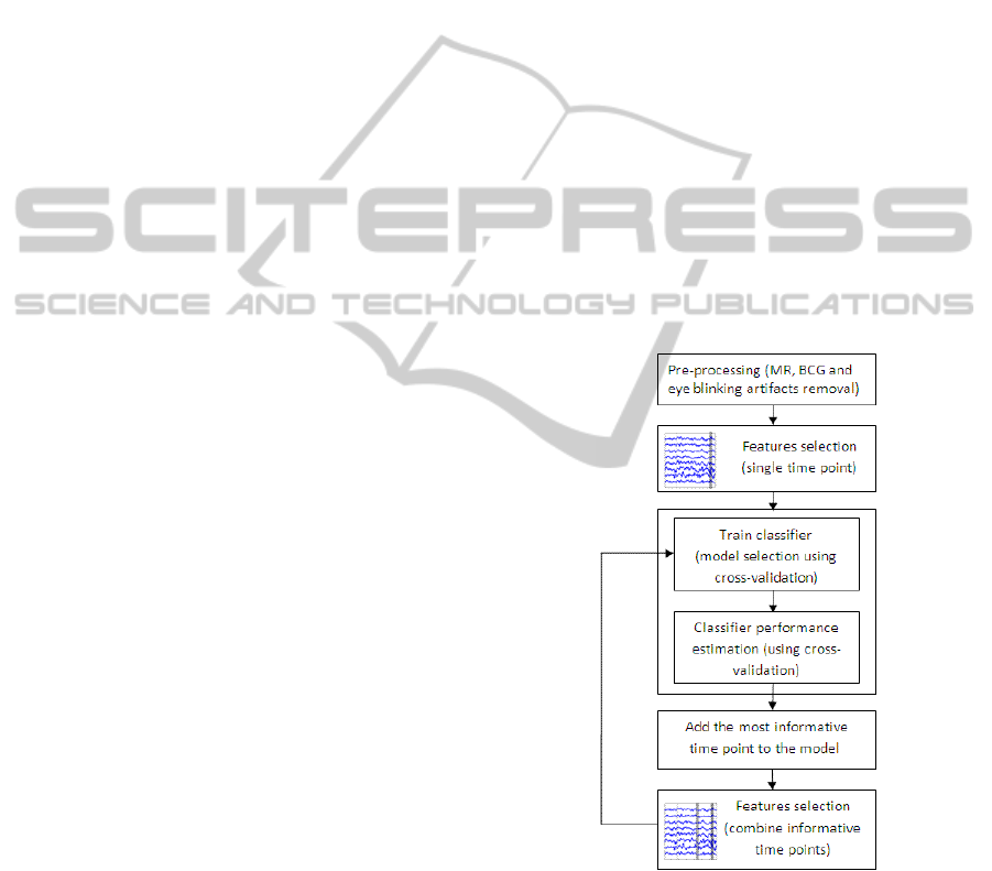
temporal analysis. Figure 1 shows the flowchart of

the ensemble method.

Figure 1: Brain state modelling flow chart.

The essence of the modelling approach is creating a

parametric family of classifiers and seeking an

optimal member of this family by model selection

techniques. The parameter which forms the

collection of classifiers controls the bias/variance

tradeoff (i.e. regularization parameter), thus a

classifier with optimal bias/variance is chosen

INFERENCE OF BRAIN MENTAL STATES FROM SPATIO-TEMPORAL ANALYSIS OF EEG SINGLE TRIALS

(Geman and Bienenstock, 1992). Each member of

the family attempts to predict the mental states of the

brain by finding the coefficients of the model which

mostly differentiate the EEG data into two mental

states. The selection of the optimal member is done

based on the classifier ability to predict the mental

states of the brain.

3.1 Model Estimation

Cross-validation is used for choosing the best model

and estimating its predictive accuracy. This method

is computationally expensive but is especially

important when the number of samples is small.

Cross-validation is applied twice: first for dividing

the original data into train and test sets. We search

for the optimal model on the train sets and check its

accuracy on the test sets. For this we used m-k-fold

cross validation, where k is the number of unique

test sets, and m is the number of times, this process

is repeated. Second, an additional inner n-fold

cross-validation procedure is applied for selecting

the optimal model on the training sets, where n is the

number of averaged cross-validation iterations.

In the first cross validation procedure, the original

data is partitioned into k disjoint sets. A single

dataset is retained as the test data for testing the

model, and the remaining k − 1 disjoint datasets are

used as training data. The cross-validation process is

then repeated k times, with each of the k sets used

exactly once as the test data. We repeat this process

m times. The training sets are used for choosing the

best model and the test sets are used to check its

predictive accuracy. The predictive accuracy of the

model is defined as the number of wrongly predicted

samples divided by the overall number of samples.

The second cross-validation operation is used for

choosing the optimal model. The training dataset is

randomly splitted, n times, into 80-20% training and

validation sets respectively. The classifier runs on

the training set with different values of the

regularization parameter (within the range of

interest) and selects the one that yields the best

results (i.e. bring mean square error, MSE, to

minimum) (see Figure 2).

The range of regularization values of interest is

determined using the singular values, which are

obtained from SVD decomposition of the processed

data matrix (used for training and testing). The range

is bounded between the minimal and the maximal

singular values. For computational efficiency, the

actual regularization values in that range are

distributed uniformly on the logarithmic scale (i.e.

the ratio of the two successive samples is constant).

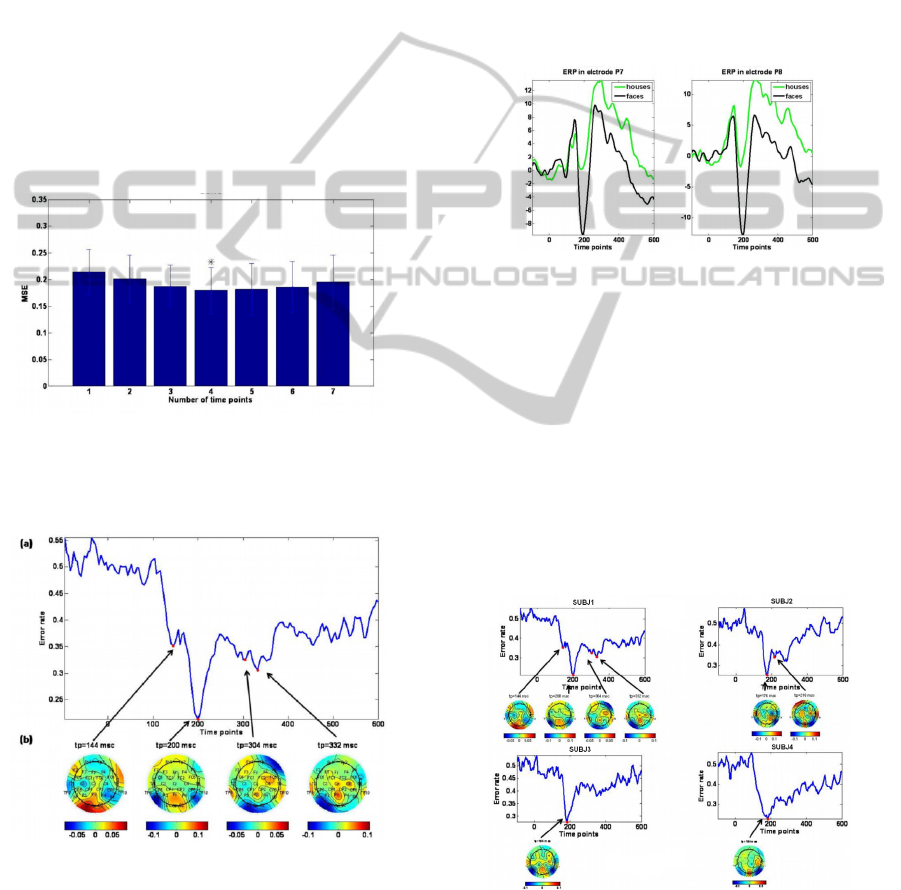
Figure 2: MSE received on the validation set at the best

time point versus the log of the regularization parameter.

The lambda that minimizes the average error across

iterations is chosen to be the optimal regularization

parameter for the model.

3.2 Regularized Logistic Regression

The proposed regularized brain state interpretation

can be used with a variety of linear and nonlinear

classifiers. The, logistic regression model is the

appropriate one for a binary classification task. It is

also optimal in terms of simplicity, interpretability

of its coefficients and speed (Hosmer and

Lemeshow

, 1989; Friedman et al., 2001).

A useful variable is the odds ratio, which is

defined as the ratio of the probability that an event

occurs to the probability that it fails. The logit (log

odds) of the logistic regression model is given by the

following equations, where

w are the model's

coefficients:

xwxwxwwxg ++

...)(

22110

(1)

)1/()()|1(

)()( xgxg

eexxYP +===

(2)

)()))(1/()(log(log xgxxodds =−

(3)

The coefficients are often estimated via the

Maximum Likelihood Estimation (MLE) method,

which seeks to maximize the log likelihood over the

entire observed data:

)|(log)(

∑

xyYPwl

(4)

The log likelihood value represents how likely the

dependent variable can be predicted from the

observed values of the independent variables.

Maximization of the above expression can be done

in various ways, most popular being the Newton-

Raphson (NR) algorithm.

The regularized version of the logistic regression

algorithm seeks to find the weights (w) which

maximizes the equation:

BIOSIGNALS 2011 - International Conference on Bio-inspired Systems and Signal Processing

wwwlwl

)()(

−=

(5)

We use the Matlab-based MVPA toolbox (Detre

et al., 2006), which implements regularized logistic

regression following notes from (Minka, 2003).

3.3 Features Selection

As mentioned before, one of the main challenges

while working with EEG signals is the high data

dimensionality. In this case, feature selection is

important for reducing the dimensionality of the

input signal, removing noise, improving learning

performance, speeding up the learning process and

improving predictive accuracy.

Feature selection is defined as the process of

choosing an optimal subset of features according to

a certain criterion. The problem of feature selection

has been extensively researched by the machine

learning/pattern recognition community over the

years (Lotte et al., 2007).

In this study, we implement a two step feature

selection algorithm. First we employ the selection of

32 electrodes from a single time point as an input for

the classifier in the same manner as in (Zhdanov et

al., 2007), second, we combine informative time-

points together as an input for the classifier.

We obtain a set of T trials labeled data samples,

each represented by NxM signal matrix, where N is

the number of channels and M is the number of time

sampling points in the segmented interval. For each

time point (from M), we create a feature vector that

contains the EEG data of the entire electrodes in this

time point. (This reduces the dimension of the data

from 32

175 to 32). Afterwards, a family of

classifiers is constructed with different

regularization parameters and applied on the

different time points. The model which achieved the

minimum MSE on the validation set, over the entire

time points, is chosen.

After selecting the model, we evaluate the

predictive accuracy of each time point using the test

sets, by applying the best model on each time point

and averaging the results. The outcome of this stage

is a ranking of the entire time points according to the

performance of the model (Figure 3). The best time

point with the lowest error rate, best separates

between the brain mental states. The coefficients of

the regression equation at the time point where

minimal prediction error is achieved indicate the

contribution of activity in different electrodes in this

time point towards the prediction. This can be

interpreted as the strength of activity in electrodes

Figure 3: (a) Predictive accuracy of each time point, on the

testing set. The black line show the average error rate over

the cross-validation iterations and the blue line represents

control results obtained using the same algorithm on data

with randomly scrambled target labels. It can be seen that

the best prediction is achieved around 200ms after the

stimulus onset (N170). (b) The coefficients of the

regression equation in the best time point. The coefficients

indicate the most contributing electrodes in this time point;

Blue color indicates strong negative effect of faces

compared to houses.

which best contributes to the mental states

separation.

The formulation presented so far indicates the

most predictive time point and the configuration of

electrodes at that time point. This spatial coding,

where the prediction depends on a configuration of

electrodes activity as a single time point, may not be

the optimal code used by the brain in interpreting the

stimuli. Therefore it is possible that a temporal or

spatio/temporal coding is more appropriate.

The presented model can address this question,

although the computational problem involved

becomes too big for a single computer to handle, but

thanks to a computer grid of several hundred

personal computers, the model can be extended in

this direction.

In this aspect we sort the local minima in the

prediction graph to find different distinct temporal

locations with prediction error minimum. The

sorting was done in an increasing order (starting

from the most predictable time point to the least

predictable time point). Then a collection of models

is applied, each using an increasing amount of

information, where new time points (electrode

information) are added into the model. In each such

input data configuration we perform the full cross-

validation estimation to estimate optimal

regularization and prediction error.

Time points were sequentially added to the model

using a wrapper algorithm (Kohavi and John, 1997),

which is a feature selection technique for selecting

an optimal subset of features from a large search

INFERENCE OF BRAIN MENTAL STATES FROM SPATIO-TEMPORAL ANALYSIS OF EEG SINGLE TRIALS

space. The features were assessed according to their

usefulness to a given predictor and added to the

subset, one by one. The ten most predictable time

points were included in this process and they were

added to the model according to their contribution to

the overall prediction.

We compared the outcome of the classifier for a

different number of time points and choose the ideal

number of time points which has significantly lower

error prediction (Figure 4). Increasing the input

vector adds electrode activity data, but also adds free

parameters to the model leading to higher chance of

overfitting the training data. We thus search for the

ideal number of time points which balances between

the two effects. Figure 5 shows the best time points

found for one subject and the electrodes activity in

these time points contributing towards mental state

discrimination.

Figure 4: prediction error vs. number of time points. For

this subject the optimal is 4, namely there was a

significant prediction improvement up to that point

(**p<0.05).

Figure 5: (a) The ideal number of time points chosen as

input for the classifier. (b) The regression coefficients

received in those time points.

4 RESULTS

4.1 Spatio-Temporal Analysis

Many studies have shown that pictures of faces elicit

a much larger ERP of negative polarity than other

object categories. This component peaks at occipital-

temporal electrode sites at about 170 ms following

stimulus onset (Bentin et al., 1996). The larger

response of the N170 complex to faces is an

undisputed observation among researchers in the

field of face processing. (Figure 6).

Figure 6: ERP in electrodes P7 and P8.

We reinforce this result using EEG single trial

classification (Figure 7). For all subjects the best

prediction achieved around 200 ms after the stimulus

onset and the electrodes that contribute to the

maximum separation between the mental states

investigated are located in the occipital area. The

coefficients obtained on single trial training

correlated to the ERP of the corresponding

electrodes. Negative coefficients indicate the ERP

for faces is lower than the ERP for houses. In

addition, both occipital electrodes (P7 and P8) are

correlated in that time point.

Figure 7: Best time points found and the coefficients in

these time points for different subjects in the houses and

faces experiment. As expected, for the entire subjects the

best prediction is achieved around 200ms after the

stimulus onset and the most activated electrodes are in the

occipital-temporal area.

BIOSIGNALS 2011 - International Conference on Bio-inspired Systems and Signal Processing

The resulting spatial-temporal weight matrix

provides a summary representation which is easily

interpretable. A result of the dimensionality

reduction, which is performed during the pre-

processing stage, where relevant time points and

electrodes are chosen, leads to simpler

computational model training. This is in contrast to

reducing the dimensionality via reducing the

sampling rate (Tomioka and Muller, 2010).

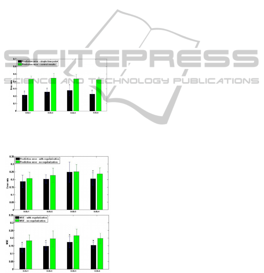
The lowest error rates achieved for each subject

using a single time point are summarized in Figure 8

(the prediction error with the optimal number of

time points is lower). The results were compared to

the control experimental results, which were

obtained using the same algorithm on randomly

scrambled labels. The difference between the mean

error estimates is significant for all subjects (P <

0.05).

Figure 8: Classification error rate for all 4 subjects. The

classification error is compared to control results obtained

using the same algorithm on randomly scrambled labels.

The difference between the mean error estimates is

significant for all subjects (*p<0.05).

Figure 9: Prediction error (Error rate and MSE) received

for 3 best time points chosen, with and without

regularization. These figures show that results with

regularization are significantly better (*p<0.05).

4.2 The Impact of Regularization

The amount of data needed to properly describe the

different mental states increases exponentially with

the dimensionality of the feature vectors. As the

amount of training data is small compared to the size

of the feature vectors, the classifier is likely to

overfit to the training data and thus producing a

model which does not uncover the true brain state

discrimination. The only way to avoid this and still

get a reliable brain state interpretation is a robust

training with a regularizer which has to be carefully

picked. To demonstrate the effect of non optimal

regularization selection, we applied the same

algorithm, with and without a regularization

parameter on feature vector of size 96 (three best

time points). As it can be seen in Figure 9, the

classification error with regularization is

significantly lower (P < 0.05).

5 CONCLUSIONS

We have proposed a robust and efficient framework

for brain state interpretation using EEG single trials.

This framework is based on extensive feature

selection using a regularized logistic regression

classifier and can be used for spatial-temporal

analysis of the EEG data. This spatial-temporal

analysis, which indicates best electrodes and best

time points, can render a far more holistic

interpretability without any a priori information on

certain optimal time points or electrode locations. It

can thus indicate whether the coding related to the

brain state discrimination task is spatial, temporal or

joint, and can indicate the network of information

propagation (at high temporal resolution) following

the stimuli. This method, which can also be applied

to a Time/Frequency representation of the signal,

can also reveal the different frequency bands at

which brain state discrimination is optimal.

ACKNOWLEDGEMENTS

This research was supported by Israeli Scientific

Foundation converging technologies program.

REFERENCES

Allison, B. Z., Wolpaw, E. W., Wolpaw, J. R., 2007. Brain

computer interface systems: progress and prospects.

Expert review of medical devices, 4 (4), pp.463-

474(12).

INFERENCE OF BRAIN MENTAL STATES FROM SPATIO-TEMPORAL ANALYSIS OF EEG SINGLE TRIALS

Bellman, R. E, 1961. Adaptive Control Processes.

Princeton University Press, Princeton, NJ.

Ben-Simon, E., Podlipsky, I., Arieli, A., Zhdanov, A.,

Hendler, T., 2008. Never resting brain: Simultaneous

representation of two alpha related processes in

humans. Plos One, 3 (12), e3984.

Bentin, S., Allison, T., Puce, A., Perez, E., McCarthy, G.,

1996. Electrophysiological studies of faces perception

in humans. Journal of Cognitive Neuroscience, 8(6),

pp. 551-565.

Blankertz, B., Dornhege, G., Krauledat, M., Müller, K. R.,

Curio, G., 2007. The noninvasive Berlin brain-

computer interface: fast acquisition of effective

performance in untrained subjects. NeuroImage, 37(2),

pp. 539–550.

Christoforou, C., Sajda, P., Parra, L. C., 2008. Second

order bilinear discriminant analysis for single trial

EEG analysis. Advances in Neural Information

Processing Systems, 20, pp. 313–320.

Delorme, A., Makeig, S., Sejnowski, T., 2001. Automatic

artifact rejection for EEG data using high-order

statistics and independent component analysis.

Proceedings of the 3rd International ICA Conference.

Detre, G., Polyn, S. M., Moore, C., Natu, V., Singer, B.,

Cohen, J., Haxby, J. V., Norman, K. A., 2006. The

Multi-Voxel Pattern Analysis (MVPA) Toolbox.

Poster presented at the Annual Meeting of the

Organization for Human Brain Mapping, Italy.

Dornhege, G., Millán, J. del R., Hinterberger, T.,

McFarland, D., Müller, K.-R. (Eds.), 2007. Towards

Brain-Computer Interfacing. MIT Press.

Duda, R. O., Hart, P. E., Stork, D. G., 2001. Pattern

Recognition 2nd edn (New York: Wiley-Interscience)

Ekman, P., Friesen, W., 1976. Pictures of facial affect,

Consulting Psychologists Press, Palo Alto, CA.

Friedman, J., Hastie, T., Tibshirani, R., 2001. The

elements of statistical learning. Springer.

Geman, S., Bienenstock , E., 1992. Neural networks and

the bias/variance dilemma. Neural Computation, 4 (1),

pp. 1–58.

Hosmer , D. W., Lemeshow, S., 1989. Applied logistic

regression. New York: John Wiley, pp. 118-24.

Jain, A. K., Duin, R.P.W.,Mao, J., 2000. Statistical pattern

recognition: a review IEEE Trans. Pattern Anal.

Mach. Intell. 22, pp.4–37

Kaper, M., Meinicke, P., Grossekathoefer, U., Lingner, T.,

Ritter, H., 2004. BCI competition 2003–data set llb:

support vector machines for the p300 speller paradigm

IEEE Trans. Biomed. Eng. 51, pp.1073–6.

Kohavi, R., John, G., 1997. Wrappers for feature subset

selection. Artificial Intelligence, 97 (1-2), pp. 273-324.

Lal, T., Schröder, M., Hinterberger, T., Weston, J.,

Bogdan, M., Birbaumer, N., Schölkopf, B., 2004.

Support vector channel selection in BCI. IEEE Trans.

Biomed. Eng., 51(6), pp. 1003–1010.

Laufs, H., Krakow. K., Sterzer. P., Eger. E., Beyerle. A.,

Salek-Haddadi. A., Kleinschmidt. A., 2003.

Electroencephalographic signatures of attentional and

cogntive default modes in spontaneous brain activity

fluctuations at rest. Proceedings of the National

Academy of Sciences, U.S.A., 100, 11053–11058.

Lehmann, D., Skrandies, W., 1980. Reference-free

identification of components of checkerboard-evoked

multichannel potential fields. Electroencephalogr Clin

Neurophysiol, 48 (6), pp. 609–621.

Lehmann, D., Ozaki, H. and Pal, I. 1987. EEG alpha map

series: brain microstates by space-oriented adaptive

segmentation. Electroenceph. clin. Neurophysiol., 67

(3), pp. 271-288.

Lotte, F., Congedo, M., Lécuyer, A., Lamarche, F.,

Arnaldi, B., 2007. A review of classifcation algorithms

for eeg-based brain-computer interfaces. Journal of

Neural Engineering, 4 (2), pp. R1.R13.

Lundqvist, D., Flykt, A., Ohman, A.,1998. The Karolinska

Directed Emotional Faces (KDEF), Department of

Neurosciences, Karolinska Hospital, Stockholm, UK.

Minka, T., 2003. A Comparison of Numerical Optimizers

for Logistic Regression. technical report, Dept. of

Statistics, Carnegie Mellon University.

Muller, T., Ball, T., Kristeva-Feige, R., Mergner, T.,

Timmer, J., 2000. Selecting relevant electrode

positions for classification tasks based on the electro-

encephalogram. Medical and Biological Engineering

and Computing, 38(1), pp. 62–67.

Murray, M. Brunet, M., Brunet, D., Michel, C. 2008.

Topographic ERP analyses: step-by-step tutorial

review. Brain Topography, 20 (4), 249–269.

Palaniappan, R., Raveendran, P., Omatu, S., 2002. VEP

optimal channel selection using genetic algorithm for

neural network classification of alcoholics. IEEE

Transactions on Neural Networks, 13(2), pp. 486–491.

Sadeh, B., Zhdanov, A., Podlipsky, I., Hendler, T., Yovel,

G., 2008. The validity of the face-selective ERP N170

component during simultaneous recording with

functional MRI. Neuroimage, 42 (2), pp.778–786.

Schröder, M., Bogdan, M., Rosenstiel, W., Hinterberger,

T., Birbaumer, N., 2003. Automated EEG Feature

Selection for Brain Computer Interfaces, Proceedings

of 1st International IEEE EMBS Conference on Neural

Engineering, Capri Island, Italy.

Tomioka, R., Aihara, K., Müller, K. R., 2007. Logistic

regression for single trial eeg classification. In:

Schölkopf, B., Platt, J., Hoffman, T. (Eds.), Advances

in Neural Information Processing Systems 19. MIT

Press, Cambridge, MA, pp. 1377–1384.

Tomioka, R., Müller, K. R., 2010. A regularized

discriminative framework for EEG analysis with

application to brain-computer interface. Neuroimage.

49 (1), pp.415-32.

Wolpaw, J. R., Birbaumer, N., McFarland, D. J.,

Pfurtscheller, G., Vaughan, T. M., 2002. Brain–

computer interfaces for communication and control

Clin. Neurophysiol. 113 (6), pp. 767–91.

Zhdanov, A., Hendler, T., Ungerleider, L., Intrator, N.,

2007. Inferring functional brain States using temporal

evolution of regularized classifiers. Comput. Intell.

Neurosci, p. 52609.

BIOSIGNALS 2011 - International Conference on Bio-inspired Systems and Signal Processing