AUTO-STEREOSCOPIC RENDERING QUALITY ASSESSMENT
DEPENDING ON POSITIONING ACCURACY OF IMAGE
SENSORS IN MULTI-VIEW CAPTURE SYSTEMS
M. Ali-Bey, S. Moughamir and N. Manamanni
CReSTIC, Reims Champagne-Ardenne University, Moulin de la Housse, BP. 1039, 51687 Reims, France
Keywords: 3DTV, Multi-view capture, Auto-stereoscopy, 3D rendering quality assessment, Accurate positioning.
Abstract: Our interest in this paper concerns the quality assessment of the 3D rendering in a production process of
auto-stereoscopic images using a multi-view camera with parallel and decentring configuration. The 3D
rendering quality problem for such process is related to the coherence of the captured images of different
viewpoints. This coherence depends, among others, on a rigorous respect of the shooting and rendering
geometries. Assuming perfect rendering conditions, we are rather interested in the shooting geometry and
image sensors positioning. This latter must be accurate enough to produce images that are quite coherent
with each other and contribute fully to achieve a quality 3D content. The purpose of this paper is precisely
to study the positioning accuracy of the different geometrical parameters of shooting based on a quality
assessment of auto-stereoscopic rendering. We propose two different approaches for assessment of the 3D
rendering quality. The first one is based on visual assessment tests of the 3D rendering quality by human
observers. The second approach is based on the acquired scientific knowledge on human visual acuity. We
present some simulation and experimental tests as well as the obtained results and their repercussion on the
positioning accuracy of the shooting parameters.
1 INTRODUCTION
Nowadays, three-dimensional television (3DTV)
knows a real revolution thanks to the technological
headways in visualization, computer graphics and
capture technologies. Depending on the technology
adopted, the 3D visualization systems can be either
stereoscopic or auto-stereoscopic. In stereoscopy,
viewing glasses are required and different
technologies are used to separate the left-eye and
right-eye views: anaglyph or colour multiplexing
(Sanders 2003), (Dubois, 2001), occultation and
polarization multiplexing (Blach, 2005), time
sequential presentation using active shuttering
glasses (Meesters, 2004). Auto-stereoscopic displays
do not need any special viewing glasses since they
are direction-multiplexed devices equipped by
parallax barriers or lenticular systems (Perlin, 2000),
(Dodgson, 2002), (Meesters, 2004).
To supply these display devices by 3D contents,
the more interesting and used methods are based on
the synthesis of multiple viewpoint images from 2D-
plus-depth data for stereoscopic display (Güdükbay,
2002) and auto-stereoscopic display (Müler, 2008).
The transformation between viewing and capturing
space with controlling perceived depth in
stereoscopic case is described in (Graham, 2001). A
generalized multi-view transformation model
between viewing and capturing space with
controlled distortion is proposed in (Prévoteau,
2010). A time varying concept of this architecture
for dynamic scenes capture is reported in (Ali-Bey,
2010a), (Ali-Bey, 2010b).
In the present paper, we are interested in
positioning accuracy of image sensors in such a
multi-view camera. The purpose is to determine the
positioning accuracy of different shooting
parameters ensuring a satisfactory 3D rendering
quality.
The works already devoted to the quality
assessment of 3D images (Benoit, 2008), (Kilner,
2009) does not suit our research goals focalised
rather on the impact of inaccurate positioning on the
rendering quality. For that we propose two
approaches helping in the determination of the
positioning accuracy. The first one is based on visual
assessment tests of 3D rendering quality by human
39
Ali-Bey M., Moughamir S. and Manamanni N..
AUTO-STEREOSCOPIC RENDERING QUALITY ASSESSMENT DEPENDING ON POSITIONING ACCURACY OF IMAGE SENSORS IN MULTI-VIEW
CAPTURE SYSTEMS.
DOI: 10.5220/0003325200390046
In Proceedings of the International Conference on Imaging Theory and Applications and International Conference on Information Visualization Theory
and Applications (IMAGAPP-2011), pages 39-46
ISBN: 978-989-8425-46-1
Copyright
c
 2011 SCITEPRESS (Science and Technology Publications, Lda.)

observers. The second one is based on human visual
acuity.
This paper is organized as follows: in Section 2,
the positioning accuracy problem is posed after
recalling the shooting/viewing geometrical process
of parallel and decentring configuration for auto-
stereoscopic rendering and deriving a simulation
scheme of this process. In Section 3, the visual
observation based method of rendering quality
assessment is presented with the used tools and the
obtained simulation results. In Section 4, the visual
acuity based method is presented with the obtained
results. We finish this work with some conclusions.
2 3D IMAGES
SHOOTING / VIEWING
GEOMETRICAL PROCESS
The Shooting/Viewing geometric process model
consists in some geometric transformations from the
capturing space to the rendering one. Thus, three
groups of parameters can be defined: a rendering
parameters group imposed by the auto-stereoscopic
display geometry, a second group defining the
geometric structure of the 3D camera model for
capturing the scene, and a third one controlling the
distortions that affect the 3D rendering. Knowing the
parameters of these three groups and the relations
between them, one can define a capturing
configuration satisfying both parameters imposed by
the visualization device and those of the wished
distortions.
Thereafter, one recalls succinctly the different
parts of this geometric process and the associated
parameters (Prévoteau, 2010). In a first part, a multi-
view rendering geometry of auto-stereoscopic
display device is presented with the viewing
parameters definition. Then, the shooting geometry
of parallel and decentred configuration is presented
defining the capture parameters. After that, relations
between capturing and viewing parameters are given
to define the distortion controlling parameters.
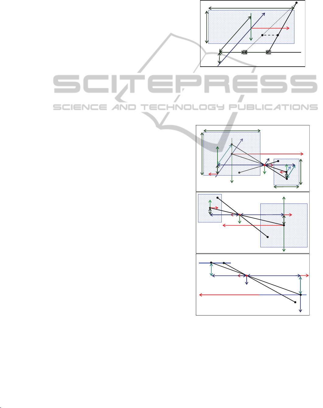
2.1 Multi-view Rendering Geometry
The considered display device is an auto-
stereoscopic screen as depicted in (Figure 1), where
H and W represent respectively the height and the
width of the device.
To perceive the 3D rendering, the observers
should be at a preferential positions imposed by the
screen and determined by a viewing distance d, a
lateral distance o
i
and a vertical distance δ
o
corresponding to a vertical elevation of the
observer’s eyes. Let b be the human binocular gap.
A viewing frame r = (C
r
, x, y, z) is associated to the
device in its centre C
r
for expressing viewing
geometry.
d
z
x
y
δ
o
m
m
i
m
ri

b
o
i
O
i
O
r
i

C
r
W
H
Figure 1: Viewing Geometry.
2.2 Shooting Geometry
The geometry of a parallel multi view shooting with
decentred image sensors configuration is presented
in (Figure 2).
Y
p
i
Z
,
Z
0
f
i
a
i
C
i
C
p
P
I
i
e
M
m
i
X
D
w
h
Hb
Wb
CB
a‐ Perspective view
Y
0
X
0
O
C
i
M
m
i
X
Y
P
p
i
a
i
e
I
i
C
p
b‐ Frontview
CB
Y
0
X
0
Y
ci
X
ci
D
f
i
I
i
C
i
M
Z
,
Z
0
m
i
X

a
i
C
p
c‐ Topview
CB
X
0
X
ci
D
Figure 2: Shooting Geometry.
IMAGAPP 2011 - International Conference on Imaging Theory and Applications
40

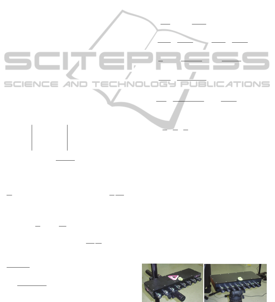
The shooting system is composed of n
sensor/lens pairs. The lenses are represented by their
optical centers C
i
and the image sensors by their
centers I
i
and their dimensions w × h. The optical
centers are aligned and uniformly distanced by an
inter-optical distance B along a parallel line to the
scene plane CB having dimensions Wb × Hb. This
scene plane is situated at a convergence distance D
from the line of optical centers. This line is elevated
by a vertical distance P regarding to the scene plane
centre C
p
. Each optical centre C
i
is defined by its
lateral position p
i
. Note that, these image planes are
coplanar and parallel to CB plane and they are also
distant by a focal length f to the optical centers line.
In addition, each image plane is decentred by a
lateral distance a
i
and a vertical distance e regarding
to the correspondent optical centre C
i
. A frame R =
(C
p
, X, Y, Z) is positioned at a chosen convergence
centre C
p
associated to the scene.
2.3 Transformation Parameters
The transition from the shooting space to the
viewing one is expressed by the transformation
between the captured point homogenous coordinates
M (X, Y, Z, 1)
R
and those of the perceived point m (x,
y, z, 1) (Prévoteau, 2010):
0
0
10
(1)
11
00
x
X
k
yY
zZ
k
d

 




  

  

  


  

  


  


(1)
Where the transformation parameters quantifying
independent distortion effects are defined as follows:
d
k
D

is the global enlargement factor,
bWb
BW
 
controls the nonlinearity of depth distortion
according to the global reduction rate
(1)
Z
k
d
    ,
b
kB
  controls the relative
enlargement width/depth rate,
Wb H
H
bW
  controls
the relative enlargement height/width rate.
ii
pb oB
dB



controls the horizontal clipping rate
and
o
BPb
dB





controls vertical clipping rate.
2.4 Specification of Multi-view
Shooting Layout
Knowing the viewing, capturing and distortion
parameters presented previously, one can specify a
capturing layout satisfying the transformations and
taking into account both the parameters imposed by
the display device (Figure 2) and the parameters of
the desired distortion k,
 ,  , ρ, γ and δ. Then, the
geometrical parameters of the specified capture
layout are pulled and expressed as follows:


,
,
,,
,
bb
bb
o
i
i
i
i
i
o
H
W
WH
kk
Wf Hf
Wf Hf
wh
Dd D d
od
d
d
DP p
kk k
fo d
pf
a
Dd
fd
Pf DF
ef
DdDF








 





 


 



 

(2)
The last relation of (2) is pulled from Descartes
relation:
111
f
DF

 and makes autofocus in order to
obtain a sharp image on each point of view, where
F
is the lens focal.
Note that to obtain a perfect 3D rendering
without distortions, it is sufficient to choose the
distortion parameters as follows:
 = 1,  = 1, ρ = 1,
γ = 0 and δ = 0.
Based on this analysis some industrial
applications such as 3D-CAM1 and 3D-CAM2
prototypes (Figure 3) were developed by our partner
3DTV-Solutions Society. These prototypes are able
to capture images of eight points of view
simultaneously and which can be displayed, after
interlacing, on an auto-stereoscopic screen in real-
time. Note however that these prototypes are
designed only for static and quasi-static scenes
presenting one constant and known convergence
distance for each prototype.
Figure 3: 3D-CAM1 and 3D-CAM2 prototypes.
AUTO-STEREOSCOPIC RENDERING QUALITY ASSESSMENT DEPENDING ON POSITIONING ACCURACY OF
IMAGE SENSORS IN MULTI-VIEW CAPTURE SYSTEMS
41

2.5 The Simulation Scheme
A simulation scheme reproducing the global
shooting/rendering geometrical process is given in
(Figure 4). It exploits a perspective projection model
based on the parameters defined above in the case of
static scenes by assuming the convergence distance
of the camera to be equal to the real distance of the
scene.
3D scene
3D
Camera
Projection
Model
Image
interlacing
Image 1
Image 2
Image n
X
Y
Z
Structural
Parameters
Calculation
B
a
i
f
P
e
D
3D screen
3D scene
3D
Camera
Projection
Model
Image
interlacing
Image 1
Image 2
Image n
X
Y
Z
Structural
Parameters
Calculation
B
a
i
f
P
e
D
3D screen
Figure 4: Simulation scheme of the production process
The obtained simulation results under
Matlab/Simulink environment are presented in
(Figure 5). The delivered 3D images and 3D videos
are visualized on an auto-stereoscopic screen
showing an optimal 3D rendering. This validates
viewing, projection and shooting geometry.
Figure 5: The eight points of view and resultant 3D image.
2.6 Positioning Accuracy Problem
of the Shooting Parameters
To obtain an optimal 3D rendering, it is necessary to
ensure that the images of the different points of view
are coherent between them. Theoretically, an
optimal coherence of these images depends on the
correspondence of each pixel of each image to a
precise position in the 3D image obtained after
interlacing. In practice, it is not possible to achieve a
zero positioning error of image sensors, so a
positioning error threshold of the shooting
parameters should be determined. Thus, the image
sensors should be positioned in a precision of a
fraction of pixel near. This pixel fraction will
penalize the quality of the 3D rendering as far as it
will be significant. Ever since, the problem is how to
specify a positioning accuracy that is sufficient to
provide a satisfactory 3D rendering quality
practically achievable?
To attempt an answer to this problem we adopt
two different approaches. The first one is based on a
visual appreciation to determine the positioning
error threshold. Moreover, this method is based on
some quantization tools using error images. It will
be presented in the next section. The second method
is based on the acquired expert knowledge on human
visual acuity. The latter represents a reference error
back-propagated through the geometrical production
process in order to specify a positioning accuracy of
the image sensors to ensure a satisfactory perceived
rendering. This method will be presented in Section
4.
3 VISUAL OBSERVATION
BASED METHOD
This method consists in soiling the various shooting
geometrical parameters by different error values.
The resulting 3D images are compared visually to a
reference 3D image obtained under ideal conditions
where the parameters of shooting are calculated
theoretically. The threshold of the error affecting
each geometrical parameter is fixed when the lack of
3D rendering quality begins to be discernible by the
observers. Moreover, to get a quantitative
appreciation of the geometrical parameters’ error
extent and their repercussion on the 3D rendering
quality, an error image is defined and then
quantified. The quantization of these error images
will serve to compare the different accuracies in
terms of numerical quantities what constitutes a
valuable tool in our study. The image error quantifi-
IMAGAPP 2011 - International Conference on Imaging Theory and Applications
42

cation consists in counting the number of the
coloured pixels to define an absolute error. A
relative error is also defined by dividing the absolute
error by the number of the coloured pixels of the
reference image. An index of quality is also defined
to express directly the rendering quality.
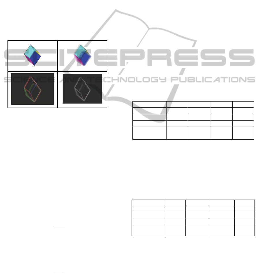
3.1 Error Images
An error image is an image produced by the
subtraction of two images
err ref
im im im. In our
case it allows the comparison of an image affected
by a positioning error of the image sensors to a
reference image obtained by a perfect positioning of
them (Figure 6):
Figure 6: Reference, current and error images.
3.2 Error Images Quantization
To quantify the error images, we adopt methods
based on counting the number of coloured pixels in
the images. To avoid redundant counting of pixels,
RGB images are converted to greyscale images
giving one matrix for each image (Figure 6). The
absolute error N
abs
is obtained by counting the
coloured pixels in the error image compared to an
image obtained with not erroneous parameters. The
relative error N
relat
is the ratio between the number of
coloured pixels in the current image error N
abs
and
the number of coloured pixels in the reference image
N
ref
at the same instant. We define it as follows:
abs
relat
ref
N
N
N

(3)
This error can be expressed also in percentage
N
relat
%= N
relat
 100. We also adopt the complement
to 1 of the relative error representing the image
quality:
1
abs
ref
N
Q
N

(4)
Thus the error is smaller when Q is closer to 1.
3.3 Repercussion
of the Shooting Parameters Error
on the Rendering Quality
In this section we are interested in the repercussion
of some shooting parameters positioning error i.e.
the inter-optical distance B, the lateral decentring a
i
and the focal length f on the 3D rendering quality.
The obtained 3D images for different positioning
errors are displayed on an auto-stereoscopic screen
and assessed visually. The corresponding quantified
errors are grouped in a table to compare the impact
of the different positioning errors on the 3D
rendering quality.
3.3.1 Error on Inter-optical Distance
For the different positioning errors committed on the
inter-optical distance B, visual assessment and
quantification of the corresponding error images are
summarized in the Table 1. The retained value of the
accuracy threshold corresponds to the satisfactory
visual assessment where ∆B = 40.6 m.
Table 1: Image quantization and visual assessment.
Error B (%) 0.5 0.1 0.05 0.01
∆B (

m)
406.3 81.2
40.6
8.12
N
relat%
(%) 0.8933 0.1790 0.1180 0.0075
Quality(Q) 0.9911 0.9982 0.9988 0.9999
Visual
Assessment
Bad
Slightly
bad
Satis-
factory
Perfect
3.3.2 Error on Lateral Decentring
In the same way, for the different positioning errors
committed on the lateral decentring a
i
, visual
assessment and quantification of the corresponding
error images are summarized in the Table 2.
Table 2: Image quantization and visual assessment.
Error a
i
(%) 0.5 0.1 0.01 0.001

a
i
(

m)
2 - 8 0.4-1.6
0.04-0.16
-
N
relat
%
(%) 0.9146 0.1934 0.0377 0
Quality (Q) 0.9909 0.9981 0.9996 1
Visual
Assessment
Bad Slightly
bad
Satis-
factory
Perfect
The retained value of the accuracy threshold
corresponds to the satisfactory visual assessment
where ai vary between 0.04 and 0.16 m according
to i leading to an average of a = 0.1m.
3.3.3 Error on Focal Length
Again, for the different positioning errors committed
AUTO-STEREOSCOPIC RENDERING QUALITY ASSESSMENT DEPENDING ON POSITIONING ACCURACY OF
IMAGE SENSORS IN MULTI-VIEW CAPTURE SYSTEMS
43

on the focal length f, visual assessment and
quantification of the corresponding error images are
summarized in the Table 3. The retained value of the
accuracy threshold of f corresponds to the
satisfactory visual assessment where ∆f = 1.72 m.
Table 3: Image quantization and visual assessment.
Error f (%) 1 0.1 0.01 0.001
∆f (m)
172 17.2
1.72
0.172
N
relat%
(%) 1.0633 0.2332 0.0302 0
Quality(Q) 0.9894 0.9977 0.9997 1
Visual
Assessment
Bad Slightly
bad
Satis-
factory
Perfect
The precisions retained in these three cases are
fixed by considering the parameters separately. By
considering them together with the retained
accuracies, the visual observation assessed the
obtained 3D rendering as satisfactory and the
quantification of the error image gives the following
values: N
ref
= 2288529 p, N
abs
= 2871 p, N
relat
=
0.0013, N
relat%
= 0.1255 %, Q = 0.9987.
Remark: This method requires significant
investment of time to perform sufficient tests to
properly determine the threshold positioning error of
each shooting parameter to ensure a satisfactory 3D
rendering. In this study we have considered a single
scene, also plenty of scenes with other conditions of
shooting should be considered to refine more the
values of positioning accuracies sought.
4 VISUAL ACUITY
BASED METHOD
The quantification of the error images were used to
compare the different accuracies and to establish
thresholds of acceptable error by using visual
assessment of the obtained 3D images, therefore,
this approach still relatively subjective.
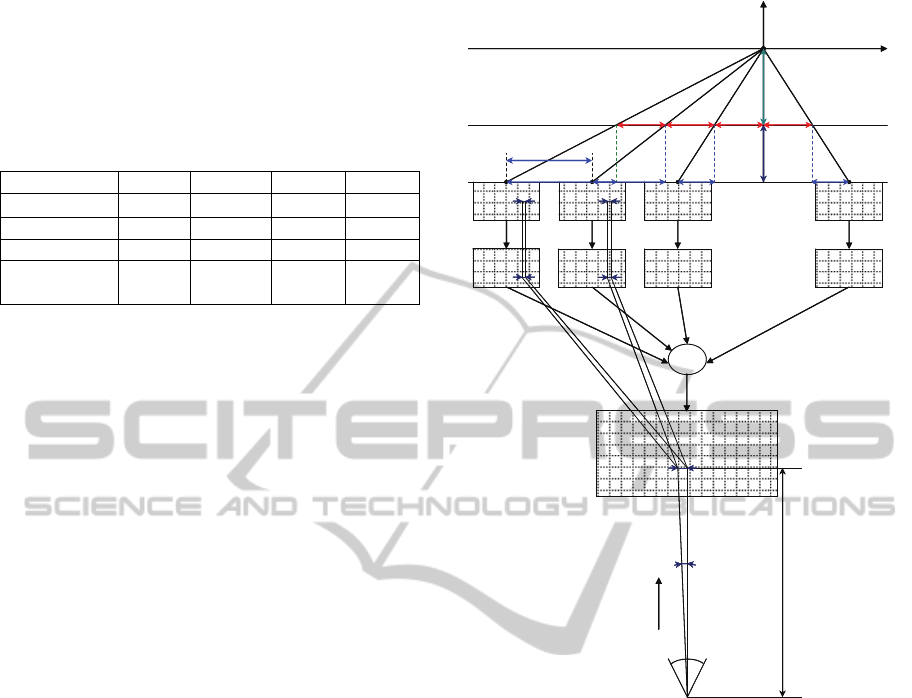
We propose in this section to establish an
objective relation between different degrees of
human visual acuity and the positioning accuracy of
the camera parameters to get a quality 3D rendering.
From the precision of human vision (visual acuity),
we'll go back up the production chain of the 3D
perception as far as the shooting parameters
positioning accuracy, through the resolution of both
a given auto-stereoscopic screen and given image
sensors (Figure 7).
Image
sensor1
Image
sensor2
Image
sensor 3
…….
Image
sensor n
Filter2 Filter3
……..
Filter n

Auto-stereoscopic screen
Observer eye
Filter1
d
α ()
BB B B
I
1
I
2
I
3
I
n
a
1
a
2
a
3
a
4
C
p
Z
D
F
E
e/2
R
e/2
C
1
C
2
C
3
C
n
Go back up
Image
sensor1
Image
sensor2
Image
sensor 3
…….
Image
sensor n
Filter2 Filter3
……..
Filter n

Auto-stereoscopic screen
Observer eye
Filter1
d
α ()
BB B B
I
1
I
2
I
3
I
n
a
1
a
2
a
3
a
4
C
p
Z
D
F
E
e/2
R
e/2
C
1
C
2
C
3
C
n
Go back up
Figure 7: 3D perception scheme of multi-view production.
4.1 Objective Relation: Visual Acuity /
Sensors Positioning Accuracy
The idea is to define a positioning error of image
sensors small enough so that a human eye with good
visual acuity is unable to detect it on the 3D image
displayed on a given auto-stereoscopic screen.
Indeed, the relation between the visual acuity
angle α and the gap E which can be detected on a
screen surface situated at a viewing distance d is
expressed as follows:
E = 2*d*tang(α/2)
(5)
This gap is equal to a proportion of the pitch of the
screen defined by:
 = E / pitch_scr
(6)
A given pixel of the image displayed on the screen
corresponds to a well-defined pixel of an image
captured by one of the n image sensors of the
camera. Thus, a pixel in one of these sensors should
not undergo a positioning error greater than:
IMAGAPP 2011 - International Conference on Imaging Theory and Applications
44

e =
 * pitch_sens
(7)
From (5), (6) and (7) we obtain the relation between
the acuity angle α and the positioning error of the
sensors:
e = 2*d*tang(α/2)*pitch_sens / pitch_scr
(8)
At this stage an objective relation between the
accuracy of sensors positioning and 3D rendering
quality expressed by the visual acuity of the
observer is derived.
4.2 Positioning Accuracy
of the Different Degree of Freedom
The questions to be answered here are: how to share
out the error e? And how to determine the
positioning accuracy of the different degree of
freedom: the inter-optical distance B, the lateral
decentring a
i
of the sensors and the focal length?
In 3D perception, each observer eye observes a
different picture of the scene. At the capturing space
level, these two images stemming from two adjacent
sensors are separated by a distance R.
The positioning error e defines the error
committed on the positioning of each pair of sensors
separated by the inter-sensor distance R defined as
follows:


1ii
R
Baa

 
(9)
The error ΔR must not exceed the value of e:
R
e
(10)
With
1ii
R
Ba a


(11)
This error can be written as follows:
1ii
aa
B
R
RR
RR


  
(12)
With
1
1
and
ii
ii
aa
B
B
Raa R
RR



    
(13)
Note that a
i
-a
i-1
is constant for all i, since R and B
have the same value for all pairs of adjacent sensors
at a given time. One can note that the quasi-totality
of the error should be endorsed to the error on B and
a tiny part is authorized as error on the lateral
decentring a
i
. This implies a maximum permissible
error on a
i
-a
i-1
of the order of 10
-3
*∆R.
This error is evenly divided on both sensors
lateral decentring, so we obtain a common value of
the absolute error:
1
()
2
ii
aa
a



(14)
Concerning the error on the focal length it is
deduced from the following relations:
() ()
***
() ()
i
i
pt Bt
afif
Dt Dt

(15)
()
()
Bt b
cste
Dt d

(16)
**
i
b
ai f
d

(17)
*
*
i
d
f
a
ib

(18)
The ratio of errors is maintained for a coherent two-
dimensional autofocus (lateral and depth), in
addition, the maximum permissible error on the
lateral decentring is the same for all points of view:
*
d
f
a
b


(19)
The error on f is thus of the order of d/b*10
-3
*∆R.
4.3 Validation using the Visual
Observation based Method
We will use the tools provided in the method based
on visual observation to evaluate the practical
validity and relevance of this second method.
We perform a test using a 30'' screen whose pitch
is 0.5025 mm and minimum viewing distance is d =
2 m. The pitch of the sensors is 3.2 m and the
considered visual acuity is
 = 1’. After calculation,
we obtain the following values: E = 0.5818 mm,
 =
1.1578, ∆R = 3.7049 m, ∆B = 3.6911 m, ∆a =
0.0097 m, ∆f = 0.2985 m.
Now by visual assessment, the 3D rendering for
acuity of 1’ is evaluated as
“perfect” and the image
error’s quantization gives the values : N
ref
= 979875
p, N
abs
= 0 p, N
relat
= 0, N
relat%
= 0 % and Q = 1.
For a 24'' screen with a pitch of 0.27 mm and a
viewing distance of 2 m, we obtain the values: E =
0.5818 mm,
 = 2.1548, ∆R = 6.8954 m, ∆B =
6.8698 m, ∆a = 0.0168 m, ∆f = 0.5179 m.
The 3D rendering is visually assessed as
“perfect” and the quantified image error values are:
N
ref
= 2294208 pixels, N
abs
= 287pixels, N
relat
=
1.2510*10
-4
, N
relat%
= 0.0125 % and Q = 0.9999.
This method is considered as severe regarding to
the applicability of the obtained results. However, a
compromise can be envisaged for a practical
solution by choosing a reasonable precision for ∆a
and ∆B. ∆f can be then deducted by calculation.
For example if we choose a precision of 0.1m
for ∆a, the accuracy of the other parameters is: ∆R =
AUTO-STEREOSCOPIC RENDERING QUALITY ASSESSMENT DEPENDING ON POSITIONING ACCURACY OF
IMAGE SENSORS IN MULTI-VIEW CAPTURE SYSTEMS
45

40.816 m, ∆B = 40.6653 m, ∆f = 3.0769 m.
The results obtained by quantifying the error
images are: N
ref
= 2294208 pixels, N
abs
= 783 pixels,
N
relat
= 3.4129 * 10
-4
, N
relat%
= 0.0341 % and
Q=0.9997 and the quality of the 3D rendering is
visually assessed as
satisfactory.
5 CONCLUSIONS
In this paper, after validating experimentally the
global shooting/viewing geometrical process for
auto-stereoscopic visualization, a visual observation
method has been proposed to assess the rendering
quality depending on the positioning accuracy of the
image sensors. Hence, a suitable accuracy is fixed
when 3D rendering is assessed to be satisfactory.
This is done with quantifying the error images to
compare the positioning error impacts of the
different structural shooting parameters.
In this method, the error images express the
inconsistency of the different viewpoint images.
Hence, with their quantification, a relation between
the images inconsistency and the visual assessment
can be achieved.
The quantification of error images and its
relation regarding to the visual assessment of the
rendering quality can constitute a basis for learning
after a sufficient number of tests. This basis will
exempt us from the visual assessment of the 3D
image quality and it will be sufficient to only use the
quantification of the error image including the
relative error.
The second proposed method provides an
objective relation between the visual acuity
expressing the quality and the positioning accuracy
of shooting parameters. This relation can be used to
specify any implying parameter (e, d, pitch of the
sensor pixels or pitch of the screen pixels) by taking
into account the other ones.
ACKNOWLEDGEMENTS
The authors thank the ANR within Cam-Relief
project and the Champagne-Ardenne region within
CPER CREATIS for their financial support.
REFERENCES
Ali-Bey M., Manamanni N., Moughamir S., 2010,
‘Dynamic Adaptation of Multi View Camera
Structure’,
3DTV-Conference: The True Vision -
Capture, Transmission and Display of 3D Video
(3DTV-CON’10),
Tampere, Finland.
Ali-Bey M, Moughamir S, Manamanni N, 2010, ‘Towards
Structurally Adaptive Multi-View Shooting System’,
18th Mediterranean Conference on Control and
Automation (MED)
, Marrakesh, Morocco.
Benoit A., Le Callet P., Campisi P., Cousseau R., 2008,
‘Quality Assessment of Stereoscopic Images’,
Hindawi, EURASIP Journal on Image and Video
Processing
. doi:10.1155/2008/659024.
Blach R., Bues M., Hochstrate J., Springer J., Fröhlich B.,
2005, ‘Experiences with multi-viewer stereo displays
based on lc-shutters and polarization’,
In Proceedings
of IEEE VR Workshop: Emerging Display
Technologies.
Dodgson N. A., 2002, ‘Analysis of the viewing zone of
multi-view autostereoscopic displays’, In Stereoscopic
Displays and Virtual Reality Systems IX
, vol. 4660 of
Proceedings of SPIE, pp. 254–265.
Dubois E., 2001, ‘A projection method to generate
anaglyph stereo images’
In Proc. IEEE Int. Conf.
Acoustics, Speech, and Signal Processing (ICASSP
'01)
, vol. 3, pp. 1661–1664, IEEE Computer Society
Press.
Graham J., Delman L., Nicolas H., David E., 2001,
‘Controlling perceived depth in stereoscopic images’,
In Proc. SPIE Stereoscopic Displays and Virtual
Reality Systems VIII
, 4297:42-53, June.
Güdükbay U., Yilmaz T., 2002, ‘Stereoscopic view-
dependent visualization of terrain height fields’, IEEE
Trans. on Visualization and Computer Graphics
, vol.
8, no. 4, pp. 330–345.
Kilner J., Starck J., Guillemaut J. Y., Hilton A., 2009,
‘Objective quality assessment in free-viewpoint video
production’, Signal Processing: Image
Communication
, vol. 24, no. 1-2, pp. 3-16.
Meesters L. M. J., Wijnand A. IJsselsteijn, Pieter J. H.
Seuntiëns, 2004, ‘A Survey of Perceptual Evaluations
and Requirements of Three-Dimensional TV’,
IEEE
Trans. on Circuits and Systems for Video Technology
,
vol. 14, no. 3, pp. 381 – 391.
Müller K., Smolic A., Dix K., Merkle P., Kauff P.,
Wiegand T., 2008, ‘View synthesis for advanced 3D
video systems’,
Hindawi Publishing Corporation,
EURASIP Journal on Image and Video Processing.
Perlin K., Paxia S., Kollin J. S., 2000, ‘An
autostereoscopic display’,
In Proceedings of the 27th
ACM Annual Conference on Computer Graphics
(SIGGRAPH '00)
, vol. 33, pp. 319–326.
Prévoteau J., Chalençon-Piotin S., Debons D., Lucas L.,
Remion Y., 2010, ‘Multi-view shooting geometry for
multiscopic rendering with controlled distortion’,
Hindawi, Int. Journal of Digital Multimedia
Broadcasting (IJDMB), Advances in 3DTV: Theory
and Practice
.
Sanders W., McAllister D. F., 2003, ‘Producing anaglyphs
from synthetic images’, In Stereoscopic Displays and
Virtual Reality Systems X
, vol. 5006 of Proceedings of
SPIE, pp. 348–358.
IMAGAPP 2011 - International Conference on Imaging Theory and Applications
46