
LINEAR MODEL FOR CANAL POOLS
Jo˜ao Miguel Lemos Chasqueira Nabais
Department of Systems and Informatics, Escola Superior de Tecnologia de Set´ubal
Campus do IPS, Estefanilha 2910-761 Set´ubal, Portugal
Miguel Ayala Botto
Department of Mechanical Engineering, IDMEC, Instituto Superior T´ecnico
Av. Rovisco Pais, 1049-001 Lisboa, Portugal
Keywords:
Modeling, Partial differential equations, Saint-Venant equations, Open-channels, Water conveyance systems,
Time delay system, Fault tolerant control.
Abstract:
Water is vital for human life.Water isused widespread from agricultural to industrial as well as simple domestic
activities. Mostly due to the increase on world population, water is becoming a sparse and valuable resource,
pushing a high demand on the design of efficient engineering water distribution control systems. This paper
presents a simple yet sufficiently rich and flexible solution to model open-channels. The hydraulic model is
based on the Saint-Venant equations which are then linearized and transformed into a state space dynamic
model. The resulting model is shown to be able to incorporate different boundary conditions like discharge,
water depth or hydraulic structure dynamics, features that are commonly present on any water distribution
system. Besides, due its computational simplicity and efficient monitoring capacity, the resulting hydraulic
model is easily integrated into safety and fault tolerant control strategies. In this paper the hydraulic model is
successfully validated using experimental data from a water canal setup.
1 INTRODUCTION
Water is an essential resource for all life species, in
particular human life. From agricultural to indus-
trial applications or simple domestic activities, an ef-
ficient water conveyance network is a key factor for
a sustainable development, social stability and wel-
fare. Water can be distributed through natural irriga-
tion canals provided by nature itself, like rivers, or
be either transported by means of artificial irrigation
canals generally known as water conveyance systems.
These systems have usually great complexity from an
automatic control point of view, since they are gen-
erally large spatially distributed systems with strong
nonlinearities and physical constraints, time delays,
while their operation typically requires the compati-
bility of multiple competing objectives. Therefore the
need for an accurate dynamic hydraulic model that
is sufficiently rich to incorporate the most relevant
physical dynamics, while being flexible enough to be
adapted to different operational setups.
For model base canal controller design is neces-
sary to have a good model able to capture the main
system dynamics. A simple analytical model was pro-
posed by (Schuurmans et al., 1995) the so-called in-
tegrator delay whose simplicity made it popular for
canal modeling (Schuurmans et al., 1999b) (Schuur-
mans et al., 1999a). Although being a simple model,
controller design using this type of model is still a cur-
rent research topic (van Overloop, 2006; Negenborn
et al., 2009). If more accuracy is needed then Saint
Venant equations (Akan, 2006) are commonly used
to model the dynamic behavior of the water flow in
open water canals. The Saint-Venant equations con-
sist of a pair of nonlinear hyperbolic partial differen-
tial equations. These equations are hard to be han-
dled and so typically a linearized version around an
equilibrium point is used for simulation and control
purposes (Litrico and Fromion, 2002). In (Litrico
and Fromion, 2009) it is shown how a continuous
multivariable dynamic model relating inflows to wa-
ter depths for an open water pool is obtained. This
model is specially suitable for H
∞
frequency anal-
ysis. Based on this structure, a simplified single-
input single-output Integral Delay Zero (IDZ) model
was shown to capture the main hydraulic dynam-
306
Miguel Lemos Chasqueira Nabais J. and Ayala Botto M..
LINEAR MODEL FOR CANAL POOLS.
DOI: 10.5220/0003536103060313
In Proceedings of the 8th International Conference on Informatics in Control, Automation and Robotics (ICINCO-2011), pages 306-313
ISBN: 978-989-8425-74-4
Copyright
c
2011 SCITEPRESS (Science and Technology Publications, Lda.)
ics (Litrico and Fromion, 2004). However, although
simple, the IDZ model lacks some accuracy (Nabais
and Botto, 2010). A more flexible model framework
that is computationally simple with efficient monitor-
ing capacity of the canal water depths is then required.
This paper presents a discrete-time linear state
space model for canal pools. The model is obtained
through the discretization of the linearized Saint-
Venant equations around a stationary point. The fol-
lowing interesting features can be found:
• a minimum computational effort is required for
simulation purposes making it easily extendable
to high dimensional open water networks;
• monitoring water depths and discharges along the
canal can be easily made through an appropriate
choice of the output equation;
• boundary conditions are easily integrated as dis-
charges or water depths, allowing for modular
interconnection of different elements on a given
open water canal;
• it enables the accommodation of hydraulic struc-
ture dynamics to which the pool is linked to;
• it can be easily integrated into model based con-
trol strategies (Martinez, 2007) (Silva et al., 2007)
opening the gate to its inclusion in fault tolerant
control applications (Blanke et al., 2006) (Iser-
mann, 2006) (Bedjaoui et al., 2009).
Besides, the proposed hydraulic model is further vali-
dated against real data retrieved from an experimental
water delivery canal hold by the NuHCC – Hydraulics
and Canal Control Center from the
´
Evora University
in Portugal.
The paper has the following structure. Section 2
presents the experimental canal. The canal model
problem formulation is then presented in section 3
where the partial differential dynamic equations de-
scribing the transport phenomenon are first linearized
and then discretized leading to a finite linear pool
model. In section 4 a brief model numerical param-
eter analysis is presented. In section 5 the hydraulic
model is validated with data retrieved from the ex-
perimental canal. Here it is shown the reliability and
accuracy of the proposed hydraulic model. Finally, in
section 6 some conclusions are drawn.
2 EXPERIMENTAL CANAL
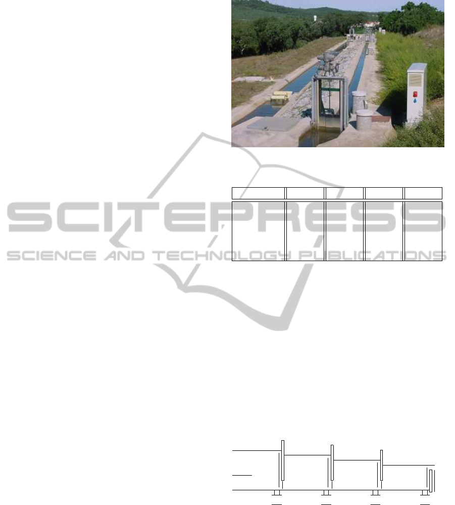
The experimental automatic canal is located in Mi-
tra near
´
Evora, Portugal (Figure 1). The canal has
4 pools with a trapezoidal cross section of 0.900m
height, 0.150m bottom width b and a side slope of
Figure 1: Experimental canal global view.
Table 1: Experimental canal uniform parameters.
Parameter Pool 1 Pool 2 Pool 3 Pool 4
L [m] 40.7 35 35 35.2
S
0
0.0016 0.0014 0.0019 0.0004
n [m
−1/3
s] 0.015 0.015 0.015 0.015
b [m] 0.15 0.15 0.15 0.15
m [m] 1:0.15 1:0.15 1:0.15 1:0.15
m = 1 : 0.15. The geometric characteristics for each
pool are shown in Table 1 where L means pool length,
S
0
the bed slope and n the Manning friction coeffi-
cient.
The 4 pools are divided by three sluice gates
as shown in Figure 2. All theses sluice gates are
electro-actuated and instrumented with position sen-
sors. A rectangular overshot gate is located at
the end of the canal with 0.38m width. The off-
take valves, equipped with an electromagnetic flow-
meter and motorized butterfly valve for flow con-
trol, are immediately located upstream of each sluice
gate. Counterweight-float level sensors are dis-
tributed along the canal.
-
Q
up
6
Y
d
1
@
@
Q
o f f
1
6
Y
g
1
6
Y
d
2
@
@
Q
o f f
2
6
Y
g
2
6
Y
d
3
@
@
Q
o f f
3
6
Y
g
3
6
Y
d
4
Z
Z
@
@
Q
o f f
4
6
Y
g
4
Figure 2: Schematics of the complete facility.
At the head of the canal an electro-valve con-
trols the canal inflow. This flow is extracted from
a reservoir. The maximum flow capacity is 0.090
m
3
/s. The flow within the automatic canal is regu-
lated by another electro-valve located at the exit of
a high reservoir (head of the automatic canal), sim-
ulating a real load situation. This high reservoir is
filled with the recovered water pumped from a low
one, which collects the flow from a traditional canal
LINEAR MODEL FOR CANAL POOLS
307

allowing a closed circuit. All electro-actuators and
sensors in the canal are connected to local PLCs
(Programmable Logic Controllers) responsible for the
sensor data acquisition and for the control actions
sent to the actuators (Almeida et al., 2002). All lo-
cal PLCs are connected through a MODBUS network
(RS 485). The interaction with the
´
Evora canal is
done through 5 inputs (canal intake Q
up
and 4 gate po-
sitions Y
g
i
), 4 outputs (downstream water level at each
poolY
L
i
) and 4 considered disturbances Q
of f
i
(offtakes
at each pool end) using a multi-platform controller in-
terface (Duarte et al., 2011).
3 CANAL POOL MODEL
3.1 First Principles
The flow in open-channels is well described by the
Saint-Venant equations,
∂Q(x,t)
∂x
+ B(x,t)
∂Y(x,t)
∂t
= 0 (1)
∂Q(x,t)
∂t
+
∂
∂x
Q
2
(x,t)
A(x,t)
+ ...
... + g· A(x,t) · (S
f
(x,t) − S
0
(x)) = 0 (2)
where, A(x,t) is the wetted cross section, Q(x,t) is
the water discharge, Y(x,t) is the water depth, B(x,t)
is the wetted cross section top width, S
f
(x,t) is the
friction slope, S
0
(x) is the bed slope, x and t are the in-
dependent variables. These equations are partial dif-
ferential equations of hyperbolic type capable of de-
scribing the transport phenomenon. The mathemati-
cal dynamical model used is known for being able to
capture the process physics namely: backwater, wave
translation, wave attenuation and flow acceleration.
To solve partial differential equations it is neces-
sary to know the initial condition along the canal axis
and also two boundary conditions in time.
3.1.1 Initial Conditions
The flow can be classified according to the indepen-
dent variables variations in time and space:
• uniform flow, when parameters do not vary along
canal axis, nonuniform when parameters vary in
space,
• steady flow, when parameters do not vary in time,
and unsteady when parameters vary in time.
In this paper the Nonuniform Unsteady Flow is as-
sumed. One interesting situation is to consider gradu-
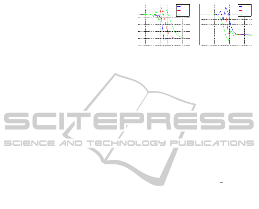
ally varied flow. This is characterized for steady con-
0 50 100 150
0
0.05
0.1
0.15
0.2
0.25
0.3
0.35
0.4
0.45
0.5
canal axis [m]
height [m]
0.8Y
N
Y
N
1.2Y
N
canal bed
Figure 3: Backwater for some downstream water depths
with a nominal discharge of Q
0
= 0.020m
3
/s.
ditions, which means
∂
∂t
= 0. In this case the Saint-
Venant equations are reduced to Ordinary Differen-
tial Equation. If also uniform flow is to be imposed,
no variations along canal axis, it is only necessary to
solve S
f
(x,t) = S
0
(x). The water depth found is also
known as the normal depth Y
N
. If a downstream wa-
ter condition different from the normal depth is given
then the water profiles presented in Figure 3 result.
3.1.2 Boundary Conditions
Partial differential equations of hyperbolic type are
capable of describing the transport phenomenon.
There are two waves presented in the pool dynamics
whose velocity are V +C and V − C, where V is av-
erage velocity across section and C is the wave celer-
ity. Depending on the relation between the dynamical
and inertial velocity captured by the Froude number,
F
r
=
V
C
the flow can be characterized into the follow-
ing three types:
• subcritical: for F
r
< 1 designated as fluvial and is
typical of large water depths and small discharge
and can be found at the river downstream,
• critical: for F
r
= 1,
• supercritical: for F
r
> 1 designated as torrential
and is typical for small depth and large discharge
and can be found at the river upstream.
In the subcritical case two waves traveling in opposite
direction along the canal axis may occur. Because
of this phenomenon, one boundary condition at each
pool end is needed. In this paper only subcritical flow
is considered.
3.2 PDE Resolution
For solving numerically the partial differential equa-
tion it is required to proceed with time and space dis-
ICINCO 2011 - 8th International Conference on Informatics in Control, Automation and Robotics
308

cretization. Here two approaches are valid (Litrico
and Fromion, 2009):
• Hydraulic approach: in this classical approach the
equations are first discretized and then the non-
linear terms are approximated. This leads to time
variant systems and requires the resolution of a
set of algebraic equations, for instance through the
generalized Newton method,
• Control approach: in this approach the equations
are first linearized around a stationary configura-
tion (Q
0
,Y
0
(x)). After this step the equations are
discretized which allows for a time invariant state
space representation.
Consider a steady state defined as (Q
0
,Y
0
(x)) where
index 0 stands for steady flow configuration. The de-
viation variables are defined as,
q(x,t) = Q(x,t) − Q
0
y(x,t) = Y(x,t) − Y
0
(x)
Assuming A(x,t) = B
0
(x)Y(x,t), after linearization
equations (1) (2) become,
B
0
(x)
∂y(x,t)
∂t
+
∂q(x,t)
∂x
= 0 (3)
∂q(x,t)
∂t
+ 2V
0
(x)
∂q(x,t)
∂x
+ δ(x)q(x,t) + ...
+
C
2
0
(x) −V
2
0
(x)
B
0
(x)
∂y(x,t)
∂x
−
˜
γ(x)y(x,t) = 0 (4)
where,
C
0
(x) =
s
g
A
0
(x)
B
0
(x)
α(x) = C
0
(x) +V
0
(x)
β(x) = C
0
(x) −V
0
(x)
δ(x) =
2· g
V
0
(x)
J
0
(x) − Fr
2
0
(x)
dY
0
(x)
dx
Fr
2
0
(x) =
V
2
0
(x)B
0
(x)
g· A
0
(x)
˜
γ(x) = V
2
0
(x)
dB
0
(x)
dx
+ g· B
0
(x)[D(x)J
0
(x) + . ..
+I(x) −
1+ 2Fr
2
0
(x)
dY
0
(x)
dx
D(x) =
7
3
−
4
3
A
0
(x)
P
0
(x)B
0
(x)
∂P
0
(x)
∂y
(5)
To complete the linearized pool model it is necessary
to consider an initial condition along the spatial coor-
dinate,
q(x,0) = q
0
(x) = q
0
y(x,0) = y
0
(x) (6)
and two boundary conditions on each end along time,
q(0,t) = u
1
(t) q(L,t) = u
2
(t) (7)
To simplify future analysis the Saint-Venant equations
can be re-written into a more convenient alternative
form. For that consider the area deviation as a(x,t) =
B
0
(x)y(x,t). The linearized equations (3) and (4) are
now given by,
∂a(x,t)
∂t
+
∂q(x,t)
∂x
= 0 (8)
∂q(x,t)
∂t
+ [α(x)− β(x)]
∂q(x,t)
∂x
+ ...
+α(x)β(x)
∂a(x,t)
∂x
+ δ(x)q(x,t) − γ(x)a(x,t) = 0 (9)
where,
γ(x) =
C
2
0
(x)
B
0
(x)
dB
0
(x)
dx
+ g[(1+ D(x))I(x) + . ..
−
1+ D(x) − (D(x) − 2)Fr
2
0
(x)
dY
0
(x)
dx
(10)
Considering the state vector χ(x,t) =
q(x,t) a(x,t)
T
equations (8) and (9) may
be expressed in state space form as follows,
A
∂
∂t
χ(x,t) + B(x)
∂
∂x
χ(x,t) +C(x)χ(x,t) = 0 (11)
where,
A =
0 1
1 0
B(x) =
1 0
α(x) − β(x) α(x)β(x)
C(x) =
0 0
δ(x) −γ(x)
(12)
3.3 Finite Dimension Model
The numerical method used to obtain a finite dimen-
sion model is the implicit method known as Preiss-
mann Scheme. In this method ∆x is the spatial mesh
dimension, ∆t is the time step, θ and φ weighting pa-
rameters ranging from 0 to 1. When using numeri-
cal methods it is important to be aware that they may
introduce nonphysical behavior that is similar to the
process physics and once introduced is not clear how
to eliminate it (Szymkiewicz, 2010).
The state vector for two consecutive sec-
tions is fourth dimension with both upstream and
downstream discharge and area deviation, x(k) =
q
k
i
a
k
i
q
k
i+1
a
k
i+1
T
, where index k stands for
time and index i stands for space. Applying the
Preissmann scheme to equation (11) after some ma-
nipulations the following discrete state space repre-
sentation is obtained,
LINEAR MODEL FOR CANAL POOLS
309
a
11
a
21
a
12
a
22
a
13
a
23
a
14
a
24
T
q
k+1
i
a
k+1
i
q
k+1
i+1
a
k+1
i+1
+ ...
... +
b
11
b
21
b
12
b
22
b
13
b
23
b
14
b
24
T
q
k
i
a
k
i
q
k
i+1
a
k
i+1
= 0 (13)
The state space representation describes the pool dy-
namics between two adjacent sections. To obtain
the model corresponding to a pool divided into N
reaches it is necessary to use N + 1 sections leading
to 2(N + 1) variables. Using model (13) is possi-
ble to obtain 2N equations. The last two equations
are related to the upstream and downstream bound-
ary conditions. The boundary conditions are imposed
normally by the structure the pool is linked to. The
boundary condition may be imposed in discharge,
usually when connected to gates, or in water depth,
when the pool is connected to large reservoirs. A
slightly more complex approach is when some hy-
draulic structure dynamics are to be incorporated into
the model. The hydraulic structure linearized equa-
tion is used as a boundary condition. In this case a
local linear model is constructed describing the pool
plus gate dynamics. With this approach the entire
open water canal dynamics can be obtained by means
of connection local model dynamics, also called lin-
ear agents. These linear agents may be used for local
model base control strategies.
In this paper discharge boundary conditions are
assumed for constructing an open water canal simu-
lator with the objective of validating the Saint-Venant
resolution method proposed.
The total pool state vector X(k) is defined as,
X(k) =
q
1
(k) a
1
(k) q
2
(k) a
2
(k) ...
... q
n
(k) a
n
(k) q
n+1
(k) a
n+1
(k)
(14)
Finally, the water pool linear model representation
can be given as,
X(k+ 1) = AX(k) + BU(k)
Y(k) = CX(k) (15)
where U(k) is the model input and Y(k) is the model
output. It is important to emphasize some features
of this model: i) the partial differential equations are
solved only by matrices multiplications; ii) the num-
ber N of reaches inside a pool defines the number of
sections N + 1 and state space variables 2(N + 1); and
iii) all state space variables are accessible through ma-
trix C in the output equation.
0 5 10 15 20 25 30 35
−1
0
1
2
3
4
5
x 10
−3
canal axis [m]
water depth deviation [m]
C
r
= 1
C
r
=1.22
C
r
= 1.5
0 5 10 15 20 25 30 35
−6
−5
−4
−3
−2
−1
0
1
2
x 10
−3
canal axis [m]
water depth deviation [m]
C
r
= 1
C
r
=1.22
C
r
= 1.5
Figure 4: Wave propagation for different time step values.
4 PARAMETER ANALYSIS
The use of numerical methods for simulation may
well introduce numerical oscillations and diffusion
which, at the worst case, can lead to instability. Nu-
merical methods are also known for introducing non
physical dynamics which are similar to the process
dynamics. After a finite dimension model is obtained,
it is then crucial to proceed with parameters analysis.
It is important to knowhow the nominal model perfor-
mance is affected by the numerical parameters. This
evaluation will be done for wave propagation along
canal axis created by imposing a positive step input
discharge at the boundary condition. The analysis is
made for the second canal pool.
The nominal model was built with the following
parameters: L = 35m N = 20, ∆x =
L
N
, ∆t → C
r
≈
1, φ = 0.5 and θ = 0.5, where C
r
means the Courant
number defined as,
C
r
= α
∆t
∆x
(16)
which can be seen as the ratio between numerical ve-
locity and kinematic velocity.
4.1 Sample Time
The sample time is one of the grid dimension pa-
rameters. Reducing it means that the numeri-
cal solution is calculated faster than the dynami-
cal velocity. As a consequence the Courant num-
ber is reduced. Different Courant numbers tested
are, C
r
=
1 1.22 1.5
or in time step ∆t =
0.835 1.02 1.25
. In Figure 4 two waves trav-
elling along canal axis for a given time instant are
shown. It is clear that the system exhibits nonphysical
oscillations that are not damped by the sample time.
Time step is not a tunable parameter. It must be
chosen to keep the Courant number close to unity in
order to have similar resolution in time and space.
Contrary to what happens in continuous systems, re-
ducing the time step does not improve the numerical
solution.
ICINCO 2011 - 8th International Conference on Informatics in Control, Automation and Robotics
310

0 5 10 15 20 25 30 35
−1
0
1
2
3
4
x 10
−3
canal axis [m]
water depth deviation [m]
θ = 0.5
θ = 0.6
θ = 0.8
0 5 10 15 20 25 30 35
−6
−5
−4
−3
−2
−1
0
1
2
x 10
−3
canal axis [m]
water depth deviation [m]
θ = 0.5
θ = 0.6
θ = 0.8
Figure 5: Wave propagation for different θ values.
10
−4
10
−2
10
0
−60
−40
−20
0
20
40
60
w [rad/s]
dB
Q(0,t) to Y(0,t)
θ = 0.5
θ = 0.6
θ = 0.8
10
−3
10
−2
10
−1
10
0
−30
−20
−10
0
10
20
30
40
w [rad/s]
dB
Q(0,t) to Y(L,t)
θ = 0.5
θ = 0.6
θ = 0.8
Figure 6: Frequency response for different θ values.
4.2 Preissmann Parameters
A centered approach in space is used, which means
φ = 0.5. Only the interpolation parameter in time θ
is changed. The centered scheme is known to be un-
conditionally stable for θ ≥ 0.5. The following values
were tested θ =
0.5 0.6 0.8
. In Figure 5 the
downstream and upstream wave propagation when a
positive discharge step is applied at the pool end is
shown.
The effect of increasing the θ parameter is similar:
numerical oscillations are eliminated at the cost of in-
troducing numerical diffusion. This interpretation can
be confirmed in the frequency response represented in
Figure 6 for the upstream discharge input.
The first natural frequency is kept almost un-
changed while the higher frequenciesare damped. Al-
though these parameters allow for numerical oscilla-
tions elimination it may introduce too much diffusion
in the model.
4.3 Space Step
The space step is related to the number of reaches
N considered in a pool. Assuming uniform space
step parameter along canal axis it is practical to use
∆x =
L
N
. If more resolution in the canal is desired
this is the parameter to change, through the number of
reaches. This is important as the space step is a con-
straint to the capacity of representing smaller waves
as well as more abrupt changes in water profile. In
Figure 7 the downstream and upstream wave propa-
gation when a positive discharge step is applied at the
0 5 10 15 20 25 30 35
0
0.5
1
1.5
2
2.5
3
3.5
x 10
−3
canal axis [m]
water depth deviation [m]
N=10
N=20
N=50
0 5 10 15 20 25 30 35
−5
−4
−3
−2
−1
0
1
x 10
−3
canal axis [m]
water depth deviation [m]
N=10
N=20
N=50
Figure 7: Wave propagation for different N values.
pool end is shown. Establishing the N parameter is a
tradeoff between accuracy and model complexity.
5 MODEL VALIDATION
The model validation is done using data collected
from the experimental canal. To emphasize the canal
monitoring ability the canal configuration with the in-
termediate gates opened is used. In this case the canal
is a single pool of 145.9m length. The initial condi-
tion used was Q
0
= 0.045m
3
/s and Y
0
(L) = 0.595m
with the associated gate opening Y
g
= 0.430m. The
linear pool model was constructed considering N =
10, θ = 0.6 and a Courant number close to unity. In
this configuration the
´
Evora canal admits two inputs,
a distant upstream discharge and a local gate opening.
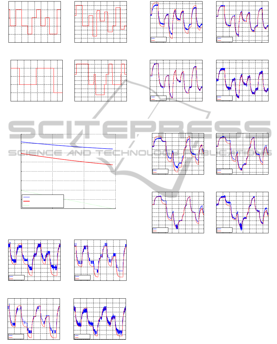
Three different input scenarios were created for
model validation, test 1 – only upstream inflow,
test 2 – only local gate opening and test 3 – with
both inputs. The scenarios run over approximately
8000s which is equivalent to 2hours and 15minutes.
The input sequence was designed accordingly to the
´
Evora canal specifications. For the inflow the interval
[0.030;0.045]m
3
/s is tested, leading to a maximum
deviation of 33% relative to Q
0
. For the gate open-
ing the interval [0.330;0.480]m is tested leading to a
maximum deviation of 23% relative to Y
0
(L). The in-
put sequence for test 3 is represented in Figure 8. In
Figure 9 the canal backwater is drawn for the upper
and lower hydraulic stationary configuration.
In Figure 10–12 the system output – the down-
stream water depth – and three more water depths
along the canal axis are shown, which proves the
model canal axis monitoring ability. One is consid-
ering x = 1/4L, x = 1/2L and x = 3/4L.
In Table 2 the error criteria for downstream wa-
ter depth as well for the intermediate points is pre-
sented. The error measurements used are the Variance
Accounted For (VAF) and the Mean Absolute Error
(MAE), the index refers to the test. The discharge in-
put causes small variation in downstream water depth
while the opening gate is more severe. The lowest
fit occurs at the downstream end, which can be ex-
LINEAR MODEL FOR CANAL POOLS
311
0 1000 2000 3000 4000 5000 6000 7000 8000
0.025
0.03
0.035
0.04
0.045
0.05
time [s]
discharge [m
3
/s]
(a) Test 1 inflow.
0 1000 2000 3000 4000 5000 6000 7000 8000
0.3
0.32
0.34
0.36
0.38
0.4
0.42
0.44
0.46
0.48
0.5
time [s]
water depth [m]
(b) Test 2 opening gate.
0 1000 2000 3000 4000 5000 6000 7000
0.025
0.03
0.035
0.04
0.045
0.05
time [s]
discharge [m
3
/s]
(c) Test 3 inflow.
0 1000 2000 3000 4000 5000 6000 7000
0.3
0.32
0.34
0.36
0.38
0.4
0.42
0.44
0.46
0.48
0.5
time [s]
water depth [m]
(d) Test 3 opening gate.
Figure 8: Tests input sequence.
0 50 100 150
0
0.1
0.2
0.3
0.4
0.5
0.6
0.7
0.8
time [s]
water depth [m]
Q=0.045l/s,Y=0.640m
Q=0.035l/s,Y=0.470m
canal bed
Figure 9: Backwater for upper and lower hydraulic steady
flow configuration during the tests.
0 1000 2000 3000 4000 5000 6000 7000 8000
0.55
0.555
0.56
0.565
0.57
0.575
0.58
0.585
0.59
0.595
0.6
time [s]
water depth [m]
experimental
simulation
(a) x = L.
0 1000 2000 3000 4000 5000 6000 7000 8000
0.52
0.53
0.54
0.55
0.56
0.57
time [s]
water depth [m]
experimental
simulation
(b) x = 3/4L.
0 1000 2000 3000 4000 5000 6000 7000 8000
0.48
0.49
0.5
0.51
0.52
0.53
0.54
0.55
time [s]
water depth [m]
experimental
simulation
(c) x = 1/2L.
0 1000 2000 3000 4000 5000 6000 7000 8000
0.45
0.46
0.47
0.48
0.49
0.5
0.51
0.52
0.53
0.54
time [s]
water depth [m]
experimental
simulation
(d) x = 1/4L.
Figure 10: Water depths for test 1.
plained by the experimental canal construction. The
0 1000 2000 3000 4000 5000 6000 7000 8000
0.48
0.5
0.52
0.54
0.56
0.58
0.6
0.62
0.64
time [s]
water depth [m]
experimental
simulation
(a) x = L.
0 1000 2000 3000 4000 5000 6000 7000 8000
0.46
0.48
0.5
0.52
0.54
0.56
0.58
0.6
0.62
0.64
time [s]
water depth [m]
experimental
simulation
(b) x = 3/4L.
0 1000 2000 3000 4000 5000 6000 7000 8000
0.46
0.48
0.5
0.52
0.54
0.56
0.58
time [s]
water depth [m]
experimental
simulation
(c) x = 1/2L.
0 1000 2000 3000 4000 5000 6000 7000 8000
0.44
0.46
0.48
0.5
0.52
0.54
0.56
0.58
time [s]
water depth [m]
experimental
simulation
(d) x = 1/4L.
Figure 11: Water depths for test 2.
0 1000 2000 3000 4000 5000 6000 7000
0.46
0.48
0.5
0.52
0.54
0.56
0.58
0.6
0.62
0.64
0.66
time [s]
water depth [m]
experimental
simulation
(a) x = L.
0 1000 2000 3000 4000 5000 6000 7000
0.44
0.46
0.48
0.5
0.52
0.54
0.56
0.58
0.6
0.62
0.64
time [s]
water depth [m]
experimental
simulation
(b) x = 3/4L.
0 1000 2000 3000 4000 5000 6000 7000
0.4
0.42
0.44
0.46
0.48
0.5
0.52
0.54
0.56
0.58
time [s]
water depth [m]
experimental
simulation
(c) x = 1/2L.
0 1000 2000 3000 4000 5000 6000 7000
0.38
0.4
0.42
0.44
0.46
0.48
0.5
0.52
0.54
0.56
time [s]
water depth [m]
experimental
simulation
(d) x = 1/4L.
Figure 12: Water depths for test 3.
canal ends with a final reach of 7m length with rectan-
gular section and 0.7m width. This is different from
the nominal parameters considered and changes the
downstream reservoir capacity.
It is important to note that while in test 1 the water
depth amplitude varies 0.030 m in test 3 due to the
gate movement, a water depth amplitude variation of
0.170 m is observed, which is quite large when com-
pared with the nominal downstream water depth.
A similar model validation was done for a model
with N = 30 which means a space step of 5m but no
increase in performance was obtained. However the
computationally cost was severely increased.
ICINCO 2011 - 8th International Conference on Informatics in Control, Automation and Robotics
312

Table 2: Model criteria error for the different tests.
Canal axis VAF
1
VAF
2
VAF
3
x = L 80.36 91.14 91.97
x = 3/4L 91.71 99.61 99.29
x = 1/2L 87.43 99.58 98.50
x = 1/4L 93.40 99.09 98.37
Canal axis MAE
1
MAE
2
MAE
3
x = L 0.0041 0.0092 0.0121
x = 3/4L 0.0066 0.0061 0.0097
x = 1/2L 0.0049 0.0019 0.0064
x = 1/4L 0.0053 0.0040 0.0074
6 CONCLUSIONS
A finite dimension linear model for canal pools has
been presented and validated with experimental data.
The linearized partial differential equations describ-
ing the system are solved through matrices multipli-
cations which requires low computational effort. This
enables the model to be used for constructing open
water network systems. The possibility to use the dis-
charge, water depth or linearized hydraulic structures
as boundary conditions, augments the model applica-
bility.
The proposed model also allows for full canal
monitoring. This is an important feature that opens
the scope of application to fault detection, isolation,
and fault tolerant control algorithms.
ACKNOWLEDGEMENTS
This work was co-sponsored by project AQUANET -
Decentralized and Reconfigurable Control for Water
delivery Multipurpose Canal Systems (PTDC/EEA-
CRO/102102/2008), FCT, Portugal, through IDMEC
by the Associated Laboratory in Energy, Transports,
Aeronautics and Space.
REFERENCES
Akan, A. O. (2006). Open Channel Hydraulics. Elsevier.
Almeida, M., ao Figueiredo, J., and Rijo, M. (2002). Scada
configuration and control modes implementation on
an experimental water supply canal. In 10th Mediter-
ranean Conference on Control Automation, Lisbon,
Portugal.
Bedjaoui, N., Weyer, E., and Bastin, G. (2009). Methods
for the localization of a leak in open water channels.
Networks and Heterogeneous Media, 4(2):180–210.
Blanke, M., Kinnaert, M., Lunze, J., and Staroswiecki,
M. (2006). Diagnosis and Fault-Tolerant Control.
Springer-Verlag.
Duarte, J., Rato, L., Shirley, P., and Rijo, M. (2011). Multi-
platform controller interface for scada application. In
IFAC World Congress (Accepted in), Milan, Italy.
Isermann, R. (2006). Fault-Diagnosis Systems. Springer-
Verlag.
Litrico, X. and Fromion, V. (2002). Infinite dimensional
modelling of open-channel hydraulic systems for con-
trol purposes. In 41th IEEE Conference on Decision
and Control, pages 1681–1686, Las Vegas, Nevada.
Litrico, X. and Fromion, V. (2004). Simplified modeling
of irrigation canals for controller design. Journal of
Irrigation and Drainage Engineering, 130:373–383.
Litrico, X. and Fromion, V. (2009). Modeling and Control
of Hysrosystmes. Springer-Verlag.
Martinez, C. A. O. (2007). Model Predictive Control of
Complex Systems including Fault Toelrance Capabil-
ities: Application to Sewer Networks. PhD thesis,
Technical University of Catalonia.
Nabais, J. and Botto, M. A. (2010). Qualitative compar-
ison between two open water canal models. In 9th
Portuguese Conference on Automatic Control, pages
501–506, Coimbra, Portugal.
Negenborn, R., van Overloop, P.-J., Keviczky, T., and
de Schutter, B. (2009). Distributed model predictive
control of irrigation canals. Networks and Heteroge-
neous Media, 4(2):359–380.
Schuurmans, J., Bosgra, O., and Brouwer, R. (1995). Open-
channel flow model approximation for controller de-
sign. Applied Mathematical Modelling.
Schuurmans, J., Clemmens, J., S.Dijkstra, Hof, A., and
Brouwer, R. (1999a). Modeling of irrigation and
drainage canals for controller design. Journal of Ir-
rigation and Drainage Engineering, 125(6):338–344.
Schuurmans, J., Hof, A., S.Dijkstra, Bosgra, O., and
Brouwer, R. (1999b). Simple water level controller
for irrigation and drainage canals. Journal of Irriga-
tion and Drainage Engineering, 125(4):189–195.
Silva, P., Botto, M. A., and ao Figueiredo, J. (2007). Model
predictive control of an experimental canal. In Eu-
ropean Control Conference, pages 2977–2984, Kos,
Greece.
Szymkiewicz, R. (2010). Numerical Modeling in Open
Channel. Springer-Verlag.
van Overloop, P. (2006). Model Predictive Control on Open
Water Systems. IOS Press.
LINEAR MODEL FOR CANAL POOLS
313
