
NESTING DISCRETE PARTICLE SWARM OPTIMIZERS FOR
MULTI-SOLUTION PROBLEMS
Masafumi Kubota and Toshimichi Saito
Faculty of Science and Engineering, Hosei University, 184-8584 Tokyo, Japan
Keywords:
Swarm inteligence, Discrete particle swarm optimizers, Multi-solution problems.
Abstract:
This paper studies a discrete particle swarm optimizer for multi-solution problems. The algorithm consists of
two stages. The first stage is global search: the whole search space is discretized into the local sub-regions
each of which has one approximate solution. The sub-region consists of subsets of lattice points in relatively
rough resolution. The second stage is local search. Each subregion is re-discretized into finer lattice points
and the algorithm operates in all the subregions in parallel to find all approximate solutions. Performing basic
numerical experiment, the algorithm efficiency is investigated.
1 INTRODUCTION
The particle swarm optimizer (PSO) is a simple
population-based optimization algorithm and has
been applied to various systems (Wachowiak et al.,
2004) (Garro et al., 2009) (Valle et al., 2008): signal
processors, artificial neural networks, power systems,
etc. The PSO has been improved and evolved in or-
der to expand the search function for various prob-
lems (Engelbrecht, 2005): multi-objective problems,
multi-solution problems (MSP), discrete PSO, hard-
ware implementation, etc. The MSP is inevitable in
real systems and several methods have been studied
(Parsopoulos and Vrahatis, 2004). The discrete PSO
operates in discrete-valuedsearch space (Engelbrecht,
2005), (Sevkli and Sevilgen, 2010)and has several ad-
vantages on reliable operation, reproducible results,
robust hardware implementation, etc. However, there
exist not many works of digital PSO for the MSP.
This paper presents the nesting discrete parti-
cle swarm optimizers (NDPSO) for the MSP. The
NDPSO consists of two stages. The first stage is
the global search. The whole search space is dis-
cretized into the local subregions (LSRs) that consist
of subsets of lattice points in relatively rough resolu-
tion. Applying the particles with ring topology, the
NDPSO tries to find the LSRs each of which includes
the first approximate solution (AS1) that is a solu-
tion candidate. The second stage is the local search
where each LSR is discretized into finer lattice points.
The NDPSO operates in all the LSRs in parallel and
tries to find all the approximate solutions (AS2). The
roughness in the global search is a key to find all AS2s
and the parallel processing in the local search is basic
for effective computation. Since the NDPSO adopts
subdivision, we have used the word ”nesting”. The
NDPSO may be regarded as a discrete version of the
multi-population method (Yang and Li, 2010) with an
eagle strategy (Yang and Deb, 2010). Performing ba-
sic numerical experiments, the algorithm capability is
investigated.
2 NESTING DISCRETE PSO
For simplicity, we consider the MSP in 2-dimensional
objectivefunctionsF(x) ≥ 0, x ≡ (x
1
,x
2
) ∈ R
2
where
the minimum (optimal) value is normalized as 0. F
has multiple solutions x
i
s
, i = 1 ∼ M: F(x
i
s
) = 0,
x
i
s
= (x
i
s1
,x
i
s2
) ∈ S
0
. The search space is normal-
ized as the center at the original with width A: S
0
≡
{x| |x
1
| ≤ A, |x
2
| ≤ A}. As a preparation, we define
several objects. The particle α
i
is described by its po-
sition x
i
and velocity v
i
: α
i
= (x
i
,v
i
), x
i
≡ (x
i1
,x
i2
),
v
i
≡ (v
i1
,v
i2
)) and i = 1 ∼ N. The position x
i
is a
potential solution. The personal best of the i-th par-
ticle, pbest
i
= F(x
pbest
i
), is the best of F(x
i
) in the
past history, The local best, lbest
i
= F(x
lbest
i
), is the
best of the personal best pbest
i
for the i-th particle and
its neighbors. For example, the neighbor means the i-
th and both sides particles in the ring topology. The
global best gbest is the best of the personal bests and
is the solution of the present state. In the complete
263
Kubota M. and Saito T..
NESTING DISCRETE PARTICLE SWARM OPTIMIZERS FOR MULTI-SOLUTION PROBLEMS.
DOI: 10.5220/0003623102630266
In Proceedings of the International Conference on Evolutionary Computation Theory and Applications (ECTA-2011), pages 263-266
ISBN: 978-989-8425-83-6
Copyright
c
2011 SCITEPRESS (Science and Technology Publications, Lda.)
graph, the lbest
i
is consistent with gbest.
First, the search space S
0
is discretized into m
1
×
m
1
lattice points as shown in Fig. 1 (a): L
0
≡
{0
11
,l
02
,··· , l
0m
1
}, l
0k
= −A+ kd − d/2, d = 2A/m
1
where k = 1 ∼ m
1
, F(x) is sampled on the discretized
search space D
0
. The target is the AS1 defined by
F(p) < C
1
, p ≡ (p
1
, p
2
) ∈ D
0
(1)
whereC
1
is the criterion. The AS1 is used to make the
LSRs each of which includes either solution. Let t
1
denote the discrete time in this stage and let k
1
denote
the counter of AS1.
Step 1. Let t
1
= 1 and let k
1
= 0. Let N
1
particles
form ring topology. The particle positions x
i
, i = 1 ∼
N, are assigned on D
0
randomly following uniform
distribution on D
0
(Fig. 1 (a)). v
i
, pbest
i
and lbest
i
are all initialized.
Step 2. The position and velocity are updated.
v
i
(t
1
+ 1) = ωv
i
(t
1
) + r
1
(x
pbest
i
− x
i
(t
1
))
+ r
2
(x
lbest
i
− x
i
(t
1
))
x
i
(t
1
+ 1) = x
i
(t
1
) + v
i
(t
1
+ 1)
(2)
where r
1
and r
2
are random parameters in [0,c
1
] and
[0,c
2
], respectively. If x
i
(t
1
+ 1) exceeds D
0
then it
is re-assigned into D
0
. The parameters ω, r
1
, r
2
, c
1
and c
2
are selected from lattice points to satisfy the
condition x(t
1
)inD
0
.
Step 3. The personal and local bests are updated:
x
pbesti
= x
i
(t
1
) if F
1
(x
i
(t
1
)) < F
1
(x
pbest
i
)
x
lbest
i
= x
pbest
i
if F
1
(x
pbest
i
) < F
1
(x
lbest
i
)
(3)
Step 4. If F(x
i
) < C
1
for some i (Fig. 1(b)) then x
i
is declared as the k
1
-th AS1 and the counter number
is increased: p
k
1
= x
i
and k
1
= k
1
+ 1. The position
x
i
is declared as a tabu lattice point and is prohibited
to revisit. x
i
is reset to a lattice point (Fig. 1(c)). v
i
,
pbest
i
and lbest
i
are all reset.
Step 5. Let t
1
= t
1
+ 1, go to Step 2 and repeat until
the maximum time step t
max1
.
In order to make the LSRs each of which is desired
to include the target solution, we select top K of the
AS1s p
1
,··· , p
K
such that F(p
1
) ≤,··· , ≤ F(p
K
) ≤
C
1
. (If k
1
< K then the top k
1
is used). Using the
AS1s, we construct subsets (LSR candidates) succes-
sively for i = 1 to K: the i-th subset S
i
is centered at
p
1
with area (2m
a
d)
2
: S
i
= {x | |x
1
− p
i
1
| < a
1
, |x
2
−
p
i
2
| < a
1
}, a
1
= m
a
d, i = 1 ∼ K where p
i
= (p
i
1
, p
i
2
) is
the i-th AS1 and m
a
is an integer smaller sufficiently
than m
1
. The m
a
determines area of S
i
in square
shape. Although this paper uses square-shaped sub-
spaces for simplicity, a variety of shapes should be
tried depending on objectiveproblems. If two or more
subsets overlaps then the subset centered at the small-
est AS1 is survivedand the other subsets are removed.
2
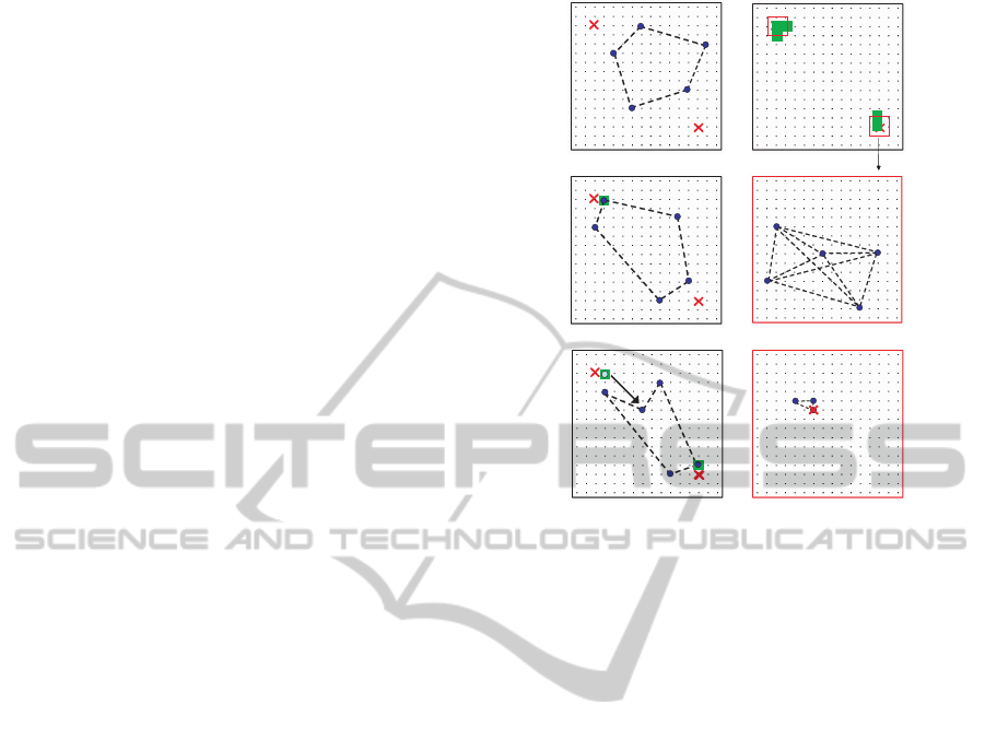
x
(a) t
1
=0
Sol1
Sol2
(b)
1
x
(c)
(d) t
1
=t
max1
2
x
1
x
(e) t
2
=0
(f)
Sol2
2
x
(a) t
1
=0
Sol1
Sol2
(b)(b)
1
x
(c)(c)
(d) t
1
=t
max1
2
x
1
x
(e) t
2
=0
1
x
(e) t
2
=0
(f)(f)
Sol2
Figure 1: Particles movement for two solutions. (a) Initial-
ization, (b) the first AS1, (c) position reset, (d) two LSRs.
(e) initialization for local search, (f) AS2.
If we obtain more than M survived subsets, we select
subsets centered at top M of AS1s. We then obtain M
pieces of LSRs and reassign the notation p
i
≡ (p
1
1
, p
i
2
)
to the AS1 in the i-th LSR. If the LSRs include the tar-
get solutions x
i
s
, i = 1 ∼ M then the global search is
said to be successful.
Next, we discretize each LSR onto m
2
× m
2
lat-
tice points: D
i
= {x | x
1
− p
i
1
∈ L
i
, x
2
− p
i
2
∈ L
i
},
L
i
= {l
i1
,··· , l
im
2
}, l
ik
= −(m
a
+ 1/2)d + kd
1
, d
1
≡
2m
a
d/m
2
This D
i
is the i-th discretized LSR. F(x) is
sampled on D
i
. The target is the AS2 defined by
F(q
i
) < C
2
, q
i
≡ (q
i
1
,q
i
2
) ∈ D
i
(4)
where C
2
(< C
1
) is the criterion. The local search
operates in parallel in D
i
(Fig. 1 (e) (f)).
Step 1. Let t
2
denote the discrete time and let t
2
= 1.
Positions of N
2
particles in complete graph are as-
signed randomly on D
i
(Fig. 1 (e)). v
i
, pbest
i
and
gbest are all initialized.
Step 2. The position and velocity are updated.
v
i
(t
2
+ 1) = ωv
i
(t
2
) + r
1
(x
pbest
i
− x
i
(t
2
))
+ r
2
(x
gbest
− x
i
(t
2
))
x
i
(t
2
+ 1) = x
i
(t
2
) + v
i
(t
2
+ 1)
(5)
where r
1
and r
2
are random parameter in [0,c
1
] and
[0,c
2
], respectively. If x
i
exceeds D
i
then it is re-
assigned into D
i
. The parameters ω, c
1
and c
2
are
selected to satisfy x
i
∈ D
i
.
Step 3. The personal and global best are updated:
x
pbesti
= x
i
(t
2
) if F
1
(x
i
(t
2
)) < F
1
(x
pbest
i
)
x
gbest
= x
pbest
i
if F
1
(x
pbest
i
) < F
1
(x
gbest
)
(6)
ECTA 2011 - International Conference on Evolutionary Computation Theory and Applications
264
Step 4. If F(x
gbest
) < C
2
for some i then we obtain
one AS2 and the algorithm is terminated.
Step 5. Let t
2
= t
2
+ 1, go to Step 2 and repeat until
the maximum time step t
max2
.
If the object is the AS2 only, the particles are of-
ten trapped into either solution or local minima and
are hard to solve the MSP. Our NDPSO tries to sup-
press the trapping by global search for the AS1 with
discretization (sampling) of the objective function.
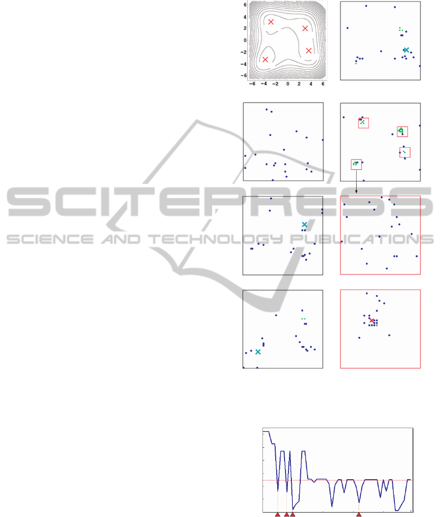
3 NUMERICAL EXPERIMENTS
In order to investigate the algorithm capability, we
have performed basic numerical experiments for the
Himmelblau function with four solutions as illus-
trated in Fig. 2 (a):
F
H
(x) = (x
2
1
+ x
2
− 11)
2
+ (x
1
+ x
2
2
− 7)
2
min(F
H
(x
i
s
)) = 0, i = 1 ∼ 4,
(7)
x
1
s
= (−2.805118,3.131312) ≡ Sol1,
x
2
s
= (3,2) ≡ Sol2,
x
3
s
= (−3.779310,−3.283185) ≡ Sol3,
x
4
s
= (3.584428,−1.848126) ≡ Sol4
S
0
= {x | |x
1
| ≤ 6, |x
2
| ≤ 6 }.
We have selected m
1
, C
1
and t
max1
as control param-
eters and other parameters are fixed after trial-and-
errors: N
1
= N
2
= 20, ω = 0.7, c
1
= c
2
= 1.4, K = 30,
m
1
/(2m
a
) = 8, m
2
= 32, t
max2
= 50 and C
2
= 0.04.
Fig. 2 (b) to (f) and Fig. 3 show a typical example
of the global search process for m
1
= 64, C
1
= 5 and
t
max1
= 50. The NDPSO find the first AS1 at t = 4
and find the other AS1s successively. At time limit
t
max1
, the NDPSO can construct all the four LSRs suc-
cessfully. Each LSR has 8
2
(8 = 2m
a
= m
1
/8) lattice
points. Fig. 2 (g), (h) and Fig. 4 show the local search
process where the NDPSO can find all the approxi-
mate solutions.
We evaluate the global search by success rate (SR)
that means rate of finding all the LSRs in 100 trials for
different initial states. Table 1 shows the SR of global
search for m
1
and C
1
. For m
1
= 32, 64 and 128, the
LSR has 4
2
, 8
2
and 16
2
lattice points, respectively in
the global search. The LSR is divided into m
2
× m
2
lattice points for the local search. We can see that
C
1
is important for finding LSRs. As C
1
increases
the SR increases and tends to saturate. For smaller
C
1
, the NDPSO operates like standard analog PSO in
principle and tends to trap local solution/minimum.
For larger C
1
, the NDPSO has possibility to find a
suitable AS1 before the trapping. As m
1
increases,
the resolution becomes higher and the SR tends to in-
crease; however, the computation cost also increases
(c) t
1
=4
2
x
1
x
6−
6−
6
6
(f) t
1
=t
max1
AS1
Sol1
Sol2
Sol3
Sol4
(a)
(b) t
1
=0
(d) t1=7
(e) t
1
=9
(g) t
2
=0
(h) t2=4
2
x
1
x
Sol3
AS1
AS1
(c) t
1
=4
2
x
1
x
6−
6−
6
6
(f) t
1
=t
max1
AS1
Sol1
Sol2
Sol3
Sol4
(a)
(b) t
1
=0
(d) t1=7
(e) t
1
=9
(g) t
2
=0
(h) t2=4
2
x
1
x
Sol3
AS1
AS1
Figure 2: Particles movement of F
H
. (a) contour map, (b)
initialization, (c) to (e) global search process, (f) four LSRs
(g) initialization for local search, (h) AS2.
1
t
1
C
0
0
10
20
40
1max
t
))((
i
pbestH
xF
mim
1
t
1
C
0
0
10
20
40
1max
t
))((
i
pbestH
xF
mim
Figure 3: Global search process of F
H
. mim(F
H
(x
i
)) means
the minimum of F
H
at time t
1
.
of course: there exists a trade-off between the SR and
computation cost.
We evaluate the local search by the SR and the
average number of iteration (#ITE) of finding all the
NESTING DISCRETE PARTICLE SWARM OPTIMIZERS FOR MULTI-SOLUTION PROBLEMS
265

)(
gbestH
xF
2
t
2
10
−
0
1.0
1
4
8
10
2
C
1
D
2
D
3
D
4
D
)(
gbestH
xF
2
t
2
10
−
0
1.0
1
4
8
10
2
C
1
D
2
D
3
D
4
D
Figure 4: Local search process of F
H
.
AS2s in 100 trials for different initial states. Table 2
shows the SR/#ITE of local search after the successful
global search. We can see that the NDPSO can find
all the AS2 speedily.
Table 1: SR of global search of F
H
for t
max1
= 50.
C
1
= 3 C
1
= 5 C
1
= 10 C
1
= 20 C
1
= 30
m
1
= 32 20 36 59 79 84
m
1
= 64 32 53 74 92 94
m
1
= 128 46 61 80 91 95
Table 2: SR/#ITE of local search of F
H
for t
max1
= 50.
C
1
= 3 C
1
= 5 C
1
= 10 C
1
= 20 C
1
= 30
m
1
= 32 100/5.30 100/5.60 100/5.46 100/5.55 100/5.57
m
1
= 64 100/5.01 100/5.34 100/5.41 100/5.43 100/5.49
m
1
= 128 100/5.08 100/5.20 100/5.36 100/5.42 100/5.55
Table 3: SR of global search of F
H
for C
1
= 5.
m
1
= 32 m
1
= 64 m
1
= 128
t
max1
= 10 8 8 8
t
max1
= 30 31 40 47
t
max1
= 50 36 53 61
t
max1
= 100 - 57 70
t
max1
= 200 - 60 71
t
max1
= 400 - - 71
t
max1
= 800 - - 72
Table 3 showsthe SR in global search for t
max1
and
m
1
. The SR increases as t
max1
increases. For m
1
= 64
and 128, the SR saturates and t
max1
= 50 (or 100) is
sufficient for reasonable results. The parameter t
max1
can control the SR and computation costs.
4 CONCLUSIONS
The NDPSO is presented and its capability is investi-
gated in this paper. Basic numerical experiments are
performed and the results suggest the following.
1. The parameters m
1
and C
1
can control rough-
ness in the global search that is important to find all
the LSRs successfully. Higher resolution encourages
trapping and suitable roughness seems to exist.
2. Parallel processing of the local search in LSRs
is basic for efficient search. If LSRs can be con-
structed, the AS2s can be found speedily and steadily.
3. The discretization is basic to realize reliable
and robust search in both software and hardware.
Future problems are many, including analysis
of search process, analysis of role of parameters,
comparison with various PSOs (Engelbrecht, 2005)
(Miyagawa and Saito, 2009) and application to prac-
tical problems (Valle et al., 2008) (Kawamura and
Saito, 2010).
REFERENCES
Engelbrecht, A. P. (2005). Fundamentals of computational
swarm intelligence. Willey.
Garro, B. A., Sossa, H., and Vazquez, R. A. (2009). Design
of artificial neural networks using a modified particle
swarm optimization algorithm. In Proc. IEEE-INNS
Joint Conf. Neural Netw., pages 938–945.
Kawamura, K. and Saito, T. (2010). Design of switching
circuits based on particle swarm optimizer and hy-
brid fitness function. In Proc. Annual Conf. IEEE Ind.
Electron. Soc., pages 1099–1103.
Miyagawa, E. and Saito, T. (2009). Particle swarm optimiz-
ers with growing tree topology. IEICE Trans. Funda-
mentals, E92-A:2275–2282.
Parsopoulos, K. E. and Vrahatis, M. N. (2004). On the
computation of all global minimizers through parti-
cle swarm optimization. IEEE Trans. Evol. Comput.,
8(3):211–224.
Sevkli, Z. and Sevilgen, F. E. (2010). Discrete particle
swarm optimization for the orienteering problem. In
Proc. IEEE Congress Evol. Comput., pages 1973–
1944.
Valle, Y., Venayagamoorthy, G. K., Mohagheghi, S., Her-
nandez, J.-C., and Harley, R. G. (2008). Particle
swarm optimization: basic concepts, variants and ap-
plications in power systems. IEEE Trans. Evol. Com-
put., 12(2):171–195.
Wachowiak, M. P., Smolikova, R., Zheng, Y., and Zurada,
J. M. (2004). An approach to multimodal biomedical
image registration utilizing particle swarm optimiza-
tion. IEEE Trans. Evol. Comput., 8(3):289–301.
Yang, S. and Li, C. (2010). A clustering particle swarm
optimizer for locating and tracking multiple optima in
dynamic environments. IEEE Trans. Evol. Comput.,
14(6):959–974.
Yang, X.-S. and Deb, S. (2010). Eagle strategy using levy
walk and firefly algorithms for stochastic optimiza-
tion. Nature Inspired Cooperative Strategies for Opti-
mization, 284:101–111.
ECTA 2011 - International Conference on Evolutionary Computation Theory and Applications
266
