GENERALIZED DISAGGREGATION ALGORITHM FOR THE

VEHICLE ROUTING PROBLEM WITH TIME WINDOWS AND

MULTIPLE ROUTES

Rita Macedo

, Sa

ıd Hanaﬁ

, Franc¸ois Clautiaux

, Cl

audio Alves

and J. M. Val

erio de Carvalho

LAMIH-SIADE, UMR 8530, Universit

e de Valenciennes et du Hainaut-Cambr

esis

Le Mont Houy, 59313 Valenciennes Cedex 9, France

Universit

e des Sciences et Technologies de Lille, LIFL UMR CNRS 8022, INRIA B

atiment INRIA

Parc de la Haute Borne, 59655 Villeneuve dAscq, France

Centro de Investigac¸

ao Algoritmi da Universidade do Minho, Escola de Engenharia, Universidade do Minho

4710-057 Braga, Portugal

Keywords:

Integer programming, Combinatorial optimization, Vehicle Routing, Network ﬂow model.

Abstract:

In this paper, we address the VRP with multiple routes and time windows. For this variant of the VRP, there is

a time interval within which every customer must be visited. In addition, every vehicle is allowed to perform

more than one route within the same planning period. Here, we propose a general disaggregation algorithm

that improves the exact approach described in (Macedo et al., 2011). We describe a novel rounding rule

and a new node disaggregation scheme based on different discretization units. We describe a new integer

programming model for the problem, which can be used, with a slight modiﬁcation, to exactly assess whether

a given solution is feasible or not. Finally, we report some computational experiments performed on a set of

instances from the literature.

1 INTRODUCTION

The vehicle routing problem (VRP) is a combinato-

rial optimization problem that was ﬁrst addressed in

(Dantzig and Ramser, 1959), as a generalization of

the traveling salesman problem. It generally consists

of scheduling vehicles to visit and deliver goods to a

set of customers. Its application area is very wide, and

there are many variants of this problem in the litera-

ture. General surveys on the VRP and its variants are

provided in (Toth and Vigo, 2002; Cordeau et al., ;

Laporte, 2009). According to (Baldacci et al., 2010),

the most effective exact approaches currently avail-

able for the classical version of the VRP are the ones

proposed in (Lysgaard et al., 2004; Fukasawa et al.,

2006; Baldacci et al., 2008).

We address the VRP with multiple routes and time

windows (MVRPTW). For this variant of the VRP,

there is a time interval within which every customer

must be visited. In addition, every vehicle is allowed

to perform more than one route within the same plan-

ning period. There are two different exact approaches

for this variant described in the literature. In (Azi

et al., 2010), the authors propose a branch-and-price

algorithm for this problem and in (Macedo et al.,

2011), a network ﬂow model embedded in an itera-

tive algorithm is described.

In this paper, we improve the algorithm proposed

in (Macedo et al., 2011). We consider a different

rounding rule and a different disaggregation of nodes.

We also generalize the previous approach and con-

sider different discretization units. Finally, we de-

scribe a new integer programming model for this

problem, which can be used, with a slight modiﬁca-

tion, to exactly assess whether a given solution is fea-

sible or not.

1.1 Problem Deﬁnition

The problem can be deﬁned in a complete graph

G = (V, A), being V its set of nodes and A = {(i, j) :

i, j ∈ V } its set of arcs. We consider that there is an

homogenous ﬂeet of k capacitated vehicles that begin

and end their routes in a single depot o. Each vehi-

cle i ∈ K = {1, . . . , k} has a capacity of Q units and

is allowed to perform more than one single route dur-

305

Macedo R., Hanaﬁ S., Clautiaux F., Alves C. and M. Valério de Carvalho J..

GENERALIZED DISAGGREGATION ALGORITHM FOR THE VEHICLE ROUTING PROBLEM WITH TIME WINDOWS AND MULTIPLE ROUTES.

DOI: 10.5220/0003755003050312

In Proceedings of the 1st International Conference on Operations Research and Enterprise Systems (ICORES-2012), pages 305-312

ISBN: 978-989-8425-97-3

 2012 SCITEPRESS (Science and Technology Publications, Lda.)

ing the planning period. This means that a vehicle

can perform a route, reload at the depot and perform

another route, until the end of the planning period,

which has a duration equal to W . The sequence of

routes and waiting times allocated to one vehicle is

deﬁned as its workday. The duration of one work-

day is, therefore, also equal to W , and the interval

[0,W ] can be seen as the depot’s opening time. This

means that vehicles can start loading from instant 0

of their workday, and that they can not arrive at the

depot after instant W. Furthermore, the maximum du-

ration between the beginning of a route and the mo-

ment that the vehicle starts to service the last customer

of that route can not be greater than t

max

. This vari-

ant specially applies to situations where vehicles per-

form short trips and are, therefore, available to per-

form more than one route per planning period. This

is, for example, the case of the delivery or collection

of perishable goods, which can not be subjected to

long trips.

For every customer i ∈ N = {1, . . . , n}, we deﬁne

, g

, s

and [a

, b

] as its demand, revenue, service

time and time window, respectively. For every arc

(i, j) ∈ A, with i, j ∈ V = N ∪ {o}, there is an asso-

ciated distance d

i j

and a traveling time t

i j

. We de-

ﬁne N

⊆ N as the subset of customers visited in route

r ∈ R, R being the set of all feasible routes. Route

r is deﬁned by a sequence of all customers in N

. It

is considered to be feasible if

∑

i∈N

≤ Q and if all

customers are visited within their time windows. For

every route r ∈ R, there is a setup time deﬁned by

∑

i∈N

, with β ∈ R

. It represents the amount of

time to be spent by the vehicle, at the depot, before it

begins the route. It is not mandatory to visit all cus-

tomers, but the number of visited customers must be

maximized.

1.2 Integer Programming Models

In what concerns integer programming models for the

MVPTW, we brieﬂy describe three models from the

literature, and propose a new one.

1.2.1 A Compact Model

In (Azi et al., 2010), the authors describe a compact

model for the MRPTW. Let x

i j

and y

be the binary

variables that determine if arc (i, j) and customer i

belong to route r ∈ R, respectively. Variable t

repre-

sents the instant at which customer i begins to be ser-

viced, in route r. The beginning and ending instants

of r are represented by t

and t

, respectively. The

constant α is a parameter that must be large enough in

order to ensure that the number of visited customers

is maximized. Let M be a sufﬁciently large number.

Finally, binary variable z

determine whether routes r

and s are consecutively performed by a same vehicle

(r < s).

min

∑

r∈R

∑

(i, j)∈A

i j

− α

∑

r∈R

∑

i∈N

(1)

s.t.

∑

j∈V

i j

= y

, ∀i ∈ N, ∀r ∈ R, (2)

∑

r∈R

≤ 1, ∀i ∈ N, (3)

∑

i∈V

−

∑

j∈V

h j

= 0, ∀h ∈ N, ∀r ∈ R, (4)

∑

i∈N

= 1, ∀r ∈ R, (5)

∑

i∈N

= 1, ∀r ∈ R, (6)

∑

i∈N

≤ Q, ∀r ∈ R, (7)

+ s

i j

− M(1 − x

i j

) ≤ t

, ∀(i, j) ∈ A,

∀r ∈ R, (8)

≤ t

≤ b

, ∀i ∈ N, ∀r ∈ R, (9)

≥ β

∑

i∈N

, ∀r ∈ R, (10)

≤ t

max

, ∀i ∈ N, ∀r ∈ R, (11)

+ M(1 − z

) ≥ t

+ β

∑

i∈N

∀r, s ∈ R, r < s, (12)

∑

r∈R

∑

s∈R|r<s

≥ |R| − k, (13)

i j

∈ {0, 1}, ∀(i, j) ∈ A, ∀r ∈ R, (14)

∈ {0, 1}, ∀i ∈ N, ∀r ∈ R, (15)

∈ {0, 1}, ∀r, s ∈ R, r < s, (16)

≥ 0, ∀i ∈ N, r ∈ R, (17)

≥ 0, ∀r ∈ R. (18)

The objective function (1) translates the objective of

maximizing the customers’ revenues, whilst minimiz-

ing the traveled distances. Customer i is visited at

most once (3) by one vehicle (2). Constraints (4) are

ﬂow conservation constraints. Every route r begins

and ends at the depot (5)-(6) and the sum of the de-

mands of all the customers in N

can not exceed the

vehicle’s capacity Q (7). All time constraints, includ-

ing traveling times (8), time windows (9), setup times

(10), (12) and maximum route durations (11), must

be respected. Finally, constraint (13) ensures that the

number of workdays does not exceed the number of

available vehicles k.

ICORES 2012 - 1st International Conference on Operations Research and Enterprise Systems

306

1.2.2 A New MIP Model

We deﬁne a new MIP model for this problem. The

set of all feasible routes R is assumed to be known.

The duration of route r is represented by σ

. Let µ

∀k ∈ K, ∀r ∈ R, be the binary variable that deﬁnes

whether route r is performed by vehicle k or not, and

be the beginning instant of route r. Variable ε

de-

ﬁnes if route r

is performed after route r. Let M be

a sufﬁciently large number. For each feasible route

r ∈ R, there is a time interval T

beg

= [T

−

, T

] that

represents the instants from which route r can begin,

in order to be feasible and to have the minimum pos-

sible duration (see section 2.2). The model states as

follows.

min

∑

r∈R

∑

k∈K

− α

∑

i∈N

(19)

s.t.

∑

k=1

≤ 1, ∀r ∈ R (20)

+ σ

≤ t

+ M(2 − µ

− µ

) + M(1 − ε

∀r, r

∈ R, (21)

+ σ

≤ t

+ M(2 − µ

− µ

) + M(1 − ε

∀r, r

∈ R, (22)

+ ε

= 1, ∀r, r

∈ R, (23)

∈ {0, 1}, ∀r ∈ R, ∀k ∈ K, (24)

∈ {0, 1}, ∀r, r

∈ R, (25)

∈ [T

−

, T

]. (26)

The objective function (19) is equivalent to the one

deﬁned in (1)-(18). Constraints (20) ensure that any

route is allocated to at most one vehicle. In order to

have a feasible solution, for every route r performed

by one vehicle, the interval ]t

+ σ

[ must be dis-

joint of any other interval ]t

+ σ

[ related to any

other route r

performed by that same vehicle. Hence,

constraints (21)-(22) ensure that ]t

+ σ

[∩]t

1.2.3 A Column Generation Model

In (Azi et al., 2010), the authors propose a branch-

and-price algorithm to solve exactly the MVRPTW.

Each column of the master problem represents one

possible workday. The set of all feasible workdays is

represented by Ω. For every workday w ∈ Ω, d

and

represent its cost and revenue, respectively. Binary

variable x

, ∀w ∈ Ω deﬁne whether or not workday w

belongs to the solution and constant a

is equal to

1 if customer i is visited in workday w. The master

problem states as follows.

min

∑

w∈Ω

− αg

(27)

s.t.

∑

w∈Ω

≤ 1, i ∈ N, (28)

∑

w∈Ω

≤ k, (29)

∈ {0, 1}, w ∈ Ω. (30)

The pricing subproblems are elementary shortest path

problems with resource constraints, which can be de-

ﬁned in a graph whose nodes correspond to feasible

routes and whose arcs deﬁne the sequencing of those

routes. They use the algorithm described in (Feillet

et al., 2004) to solve it.

1.2.4 Network Flow Model

In (Macedo et al., 2011), the authors propose

a pseudo-polynomial network ﬂow model for the

MVRPTW, which can be described as follows. Let

U be the unit discretization of the continuous inter-

val [0,W ] (see section 2.2). We deﬁne a directed

graph Π = (∆, Ψ), with ∆ = {0,U, 2U, . . . ,W } as its

set of nodes and Ψ = {(u,v)

: 0 ≤ u < v ≤ W, u ∈

beg

∩ ∆, r ∈ R}

{(u, v)

: u and v are consecutive

nodes of ∆}

{(W, 0)} as its set of arcs. Each path

of this graph corresponds to a workday to be sched-

ule to one of the available vehicles. Each node of this

graph corresponds to one time instant of the planning

period. In the ﬂow model, variables λ

represent the

ﬂow that goes through arc (u, v)

∈ Ψ, and d

stands

for the the total cost of route r ∈ R. The total ﬂow go-

ing through

∏

equals z and represents the exact num-

ber of assigned vehicles, or equivalently, the number

of deﬁned workdays in the solution. The model states

as follows.

min

∑

(u,v)

∈Ψ

− α

∑

i∈N

(31)

s.t.

∑

(u,v)

∈Ψ|i∈N

≤ 1, ∀i ∈ N, (32)

∑

(u,v)

∈Ψ

−

∑

(v,y)

∈Ψ







−z , if v = 0

0 , if v = U, . . . ,W −U,

z , if v = W

(33)

z ≤ k, (34)

≥ 0 and integer, ∀(u, v)

∈ Ψ, (35)

z ≥ 0 and integer. (36)

The objective function (31) is equivalent to the ones of

the previous models. Constraints (32) ensure that any

GENERALIZED DISAGGREGATION ALGORITHM FOR THE VEHICLE ROUTING PROBLEM WITH TIME

WINDOWS AND MULTIPLE ROUTES

307

customer is visited at most once and constraints (33)

are ﬂow conservation constraints. Finally, constraint

(34) ensures that the total ﬂow going trough the graph

does not exceed k, which means that no more than k

workdays are deﬁned and, therefore no more than k

vehicles are used.

2 IMPROVED ITERATIVE

ALGORITHM

An iterative algorithm based on model (31)-(36) has

been proposed in (Macedo et al., 2011). In this pa-

per, we investigate several improvements of this con-

vergent iterative algorithm. In (Macedo et al., 2011)

the discretization unit is constant (i.e. U = 1). We

propose a generalization by considering different dis-

cretization units for the set of nodes ∆. We also con-

sider a different rounding rule and a different disag-

gregation of nodes, and propose a new integer model

to assess exactly whether a given solution is feasible

or not. In this section, we describe these different

steps of the global algorithm.

2.1 Rounding Procedure and Possible

Infeasibilities

In (Macedo et al., 2011), the rounding strategy to

transform values u and v of every arc (u, v)

∈ Ψ into

the discrete values belonging to the set of vertices

∆ = {0, . . . ,W } of graph Π consisted of considering

u = due and v = bvc. This rounding strategy leads to

a relaxation of the problem and, therefore, its solution

represents a lower bound, which means that it may

be infeasible. In this case, infeasibities may occur

whenever there are two routes r

and r

in the solu-

tion, represented by arcs (u

, v

)

and (u

, v

)

, such

that (considering v

≤ u

, without loss of generality)

= u

or v

= u

− 1.

For our new algorithm, we use a different round-

ing strategy. We consider every value u as u =





U. This rounding procedure also leads to a relax-

ation of the problem, but it only eventually originates

one of the previous infeasibilities, for the cases where

= u

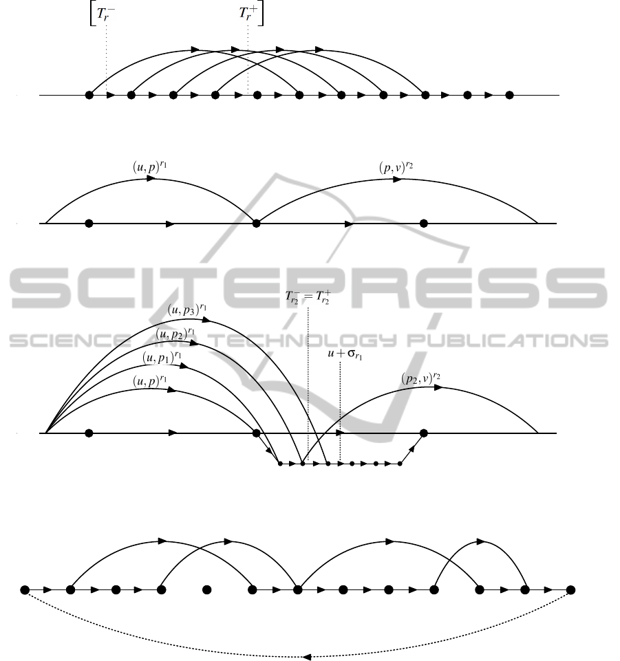
For every route r ∈ R, the arcs to consider are

arcs (u, v)

such that u ∈ (T

beg

∆)

−

×U

and v =

u + σ

. Figure 1 illustrates the arcs to

be considered for route r. In this case, given that

< T

−

< p

and p

< T

< p

(and considering

that bp

+ σ

c = p

), the arcs that represent route r

would be (p

, p

)

, (p

, p

)

, (p

, p

)

and (p

, p

)

2.2 Variable Discretization

For each feasible route r ∈ R, there is a time in-

terval T

beg

= [T

−

, T

] that represents the instants

at which route r can begin, in order to be feasible

and to have the minimum possible duration. Val-

ues T

−

and T

,∀r ∈ R, can be recursively calcu-

lated (Macedo et al., 2011). Route r beginning

at instant t is represented by r

. As explained

in (Macedo et al., 2011), route r

such that t 6∈

beg

is either infeasible or it is dominated by route

−

. The number of considered routes is there-

fore equal to

∑

r∈R

−(T

mod U))−(T

−

−(T

−

mod U))

1 . In (Macedo et al., 2011), U = 1. We now gener-

alize this concept and consider that U can take differ-

ent values. It is clear that considering U = u

rather

than U = u

, with u

> u

, implies having a smaller

model, with less variables and constraints. On the

other hand, given that with U = u

we have a coarser

rounding, the number of iterations of the algorithm

may be larger, as there is a higher probability of ob-

taining an infeasible solution. In section 3, we test,

for each instance, different values of U.

2.3 New Disaggregation Method

When the model ﬁnds a solution that is infeasible,

all nodes that are simultaneously the beginning and

the end of at least two arcs in the solution, are dis-

aggregated. To disaggregate a node p that belongs

to the original set of nodes ∆

and has not yet been

disaggregated means to consider additional nodes be-

tween p and p + U. The number of new nodes to

add depends on the chosen unit ε. Disaggregating

point p implies adding the (ε − 1) equidistant nodes



p +





, . . . , p +U −





to the graph. Whenever

there is such a node, p

∗

, that does not belong to ∆

or has already been disaggregated in a previous itera-

tion, the node to be disaggregated is the highest node

∈ ∆

, such that p

≤ p

∗

. Let ε

∗

be the distance be-

tween any two consecutive nodes in [p

, p

+U]. The

set of (aε

∗

− 1) equidistant nodes to be added to the

original graph is





aε

∗



, . . . , p

+U −



aε

∗



When nodes are added to the graph, there are ad-

ditional arcs to be considered. Figure 2 illustrates the

disaggregation of node p, and the modiﬁcations that

occur in what concerns arcs representing routes r

and

2.4 Exact Feasibility Model

A solution given by model (31)-(36) is represented by

a set of arcs. Given a set of arcs, it may be possible to

ﬁnd different solutions, as illustrated in ﬁgure (3).

ICORES 2012 - 1st International Conference on Operations Research and Enterprise Systems

308

... ...

Figure 1: Arcs representing route r.

... ...

...

p p + U

p - Up - U

p - U

Figure 2: Disaggregation of node p, with ε = 7.

0 W

r s

Figure 3: Arcs in a solution given by model (31)-(36).

For this solution, there are four routes to be performed

by two vehicles. But we can have a vehicle k

per-

forming route r

and then route s

and a vehicle v

performing route t

followed by route q

, or we can

allocate routes r

and q

to vehicle v

and routes

and s

to vehicle v

. Although the ﬁrst solution

is guaranteed to be feasible, the second solution may

not be, as node p

is simultaneously the beginning

and ending node of two routes performed by the same

vehicle.

We use model (19)-(26), with a slight modiﬁca-

tion, to assesses exactly whether it is possible or not

to build a feasible solution with the arcs of the solu-

tion, instead of only checking if one possible solution

is feasible or not.

Let R

⊆ R be the set of routes associated to

the arcs that compose the optimal solution given by

model (31)-(36). The model states as follows.

GENERALIZED DISAGGREGATION ALGORITHM FOR THE VEHICLE ROUTING PROBLEM WITH TIME

WINDOWS AND MULTIPLE ROUTES

309

min C (37)

s.t.

∑

k=1

= 1, ∀r ∈ R

, (38)

+ σ

≤ t

+ M(2 − µ

− µ

) + M(1 − ε

∀r, r

∈ R

, (39)

+ σ

≤ t

+ M(2 − µ

− µ

) + M(1 − ε

∀r, r

∈ R

, (40)

+ ε

= 1, ∀r, r

∈ R

, (41)

∈ {0, 1}, ∀r ∈ R

, ∀k ∈ K, (42)

∈ {0, 1}, ∀r, r

∈ R

, (43)

∈ [T

−

, T

], ∀r ∈ R

. (44)

The differences between model (19)-(26) and (37)-

(44) rely on constraints (38). As an input, there are

only the routes that are present in the solution given

by model (31)-(36). With this model, we want to as-

sess whether it is possible or not to build a feasible

solution with those chosen routes. That is the reason

for the equality in the constraints, as opposed to the

inequality in (19). Moreover, the objective function

(37) is not relevant, and thus we can just set it to a

constant value C. The solution found by model (31)-

(36) is feasible if and only if model (37)-(44) ﬁnds a

feasible solution for set R

2.5 Generalized Algorithm

We propose a generalization of the method described

in (Macedo et al., 2011), with some further modiﬁca-

tions. Algorithm 1) summarizes this method.

All feasible routes are implicitly generated. Graph

∏

= (∆, Ψ) is then built using the new rounding and

discretization rules described in sections 2.2 and 2.1.

We then apply all the arc reduction criteria deﬁned in

(Macedo et al., 2011), in order to increase the model’s

efﬁciency. Model (31)-(36) is solved and its solution’s

feasibility is checked by solving the exact feasibility

model (37)-(44). Whenever there is an infeasibility,

we proceed to some local node disaggregations, as de-

scribed in section 2.3, and repeat the process.

3 COMPUTATIONAL RESULTS

To investigate the effects of considering different val-

ues for the discretization unit, we conducted a set of

computational experiments on benchmark instances

from the literature. The considered instances are the

same ones described in (Azi et al., 2010; Macedo

et al., 2011).

The algorithm was implemented in C++ and the

Algorithm 1: Iterative Disaggregation Algorithm.

Input: Instance I of the MVRPTW, U, ε and a

Output: Optimal solution x

∗

Build Π = (∆, Ψ);

optimal=False;

while optimal=False do

Apply arc reduction;

Solve I with model (31)–(36), obtaining

solution x

;

Check if x

is feasible by solving model

(37)–(44);

if x

is feasible then

∗

= x

, optimal=True

else

Apply disaggregation obtaining

= (∆

, Ψ

);

Π = Π

;

network ﬂow model was solved with ILOG CPLEX

12.2. The computational tests were run on a PC with

Intel Core i7, CPU with 2.00GHz and 4GB of RAM.

The cost of a route is considered to be equal

to its traveled distance. The used parameters, de-

ﬁned in the previous sections, were set to k = 2,

α = 2max

(i, j)∈A

i j

+ 1, β = 0.2, g

= 1, ∀i ∈ N, ε = 4

and a = 2.

Table 1 reports the computational results obtained

for some of these instances, and for some different

values of U within each of the instances. We consider

values of U smaller than the minimum duration of all

routes. Columns Inst, n and t

max

refer, respectively,

to the instance’s name, the number of customers and

the value of the maximum route duration. The num-

ber of different routes is represented by |R|, and the

percentage of visited customers and optimal solution

are represented by %Cust and z

∗

. All of the values

previously described are equal for a same instance.

We then report, for each value of U, the number of

all routes, for all their beginning instances, |R

total

the number of iterations of the algorithm, n

, and

the computational time, t, in seconds. The two last

columns, %|R

total

| and %t, report the percentage of

the values of |R

total

| and t when compared to the ones

obtained with U = 1.

When the value of U increases, the total number

of routes decreases in an approximate proportion. In

what concerns the computational times, this decrease

is even more expressive, except for some cases where

the number of iterations increases considerably.

All instances are solved within the ﬁrst two iter-

ations when U = 1. For most of them, the problem

is even solved in the ﬁrst one. This had been already

observed in (Macedo et al., 2011). When the value

ICORES 2012 - 1st International Conference on Operations Research and Enterprise Systems

310

Table 1: Computational results for different values of U .

Inst n t

max

|R| %Cust z

∗

U |R

total

| n

t (s) %|R

total

| %t

RC201 25 75 92 100 988.20 1 6237 1 1.55 100.00% 100.00%

20 401 1 0.14 6.43% 9.03%

40 248 2 0.11 3.98% 7.10%

60 190 2 0.14 3.05% 9.03%

R204 25 75 922 100 579.75 1 325871 1 310.45 100.00% 100.00%

7 47163 1 4.64 14.47% 1.49%

14 23933 1 1.30 7.34% 0.42%

20 17045 1 1.16 5.23% 0.37%

C202 25 220 467 100 653.50 1 166767 1 754.30 100.00% 100.00%

7 24193 1 2.57 14.51% 0.34%

14 12300 1 0.84 7.38% 0.11%

20 8742 1 2.54 5.24% 0.34%

RC202 40 75 425 92.5 1458.09 1 67063 1 15.28 100.00% 100.00%

20 3734 5 10.72 5.57% 70.16%

40 2069 8 50.95 3.09% 333.44%

60 1498 8 42.28 2.23% 276.70%

R209 40 75 2330 100 935.95 1 284468 1 434.38 100.00% 100.00%

4 72855 3 125.88 25.61% 28.98%

7 42543 1 14.48 14.96% 3.33%

10 30604 5 68.04 10.76% 15.66%

C208 40 220 772 100 1072.22 1 258795 1 84.66 100.00% 100.00%

7 37556 1 4.22 14.51% 4.98%

14 19108 1 2.42 7.38% 2.86%

20 13609 1 1.18 3.38% 1.39%

RC207 25 100 4515 100 514.90 1 320345 1 65.30 100.00% 100.00%

20 20192 6 14.46 6.30% 22.14%

40 12326 6 13.31 3.85% 20.38%

60 9536 5 10.33 2.98% 15.82%

R202 25 100 2909 100 617.60 1 286897 1 50.98 100.00% 100.00%

7 43376 1 6.26 15.12% 12.28%

14 23102 1 3.28 8.05% 6.43%

20 17056 1 2.66 5.94% 5.22%

C207 25 250 1685 100 525.57 1 577576 1 79.39 100.00% 100.00%

7 83904 1 4.38 14.53% 5.52%

14 42847 1 2.54 7.42% 3.06%

20 30479 1 2.03 5.28% 2.33%

RC201 40 100 457 85 1157.65 1 21966 1 3.33 100.00% 100.00%

20 1542 4 1.61 7.02% 48.35%

40 997 5 1.91 4.54% 57.36%

60 818 6 4.01 3.72% 120.42%

RC205 40 100 2209 95 1195.51 1 134050 1 42.09 100.00% 100.00%

20 8786 3 3.60 6.55% 8.55%

40 5514 3 1.87 4.11% 4.44%

60 4400 3 2.09 3.28% 4.97%

C205 40 250 1153 100 921.37 1 137358 2 619.48 100.00% 100.00%

7 20518 2 4.42 14.94% 0.71%

14 10789 1 2.43 7.85% 0.39%

20 7952 1 1.85 5.79% 0.30%

GENERALIZED DISAGGREGATION ALGORITHM FOR THE VEHICLE ROUTING PROBLEM WITH TIME

WINDOWS AND MULTIPLE ROUTES

311

of U increases, the rounding becomes coarser. This

translates into a greater number of iterations for some

of the instances, although it is not always the case.

4 CONCLUSIONS

In this paper, we address a variant of the vehicle rout-

ing problem with time windows and multiple use of

vehicles. We propose an improvement of the algo-

rithm described in (Macedo et al., 2011). It mainly

consists of considering variable discretization units

for the time interval represented by the set of nodes

of the underlying graph. We also propose new round-

ing and disaggregation rules. This new algorithm was

tested with the set of instances proposed in (Azi et al.,

2010; Macedo et al., 2011). The results show consid-

erable improvements of the computational times for

most of the instances, when we increase the value of

the discretization unit.

REFERENCES

Azi, N., Gendreau, M., and Potvin, J.-Y. (2010). An ex-

act algorithm for a vehicle routing problem with time

windows and multiple use of vehicles. European Jour-

nal of Operational Research, 202(3):756 – 763.

Baldacci, R., Christoﬁdes, N., and Mingozzi, A. (2008).

An exact algorithm for the vehicle routing problem

based on the set partitioning formulation with addi-

tional cuts. Mathematical Programming, 115(2):351–

385.

Baldacci, R., Toth, P., and Vigo, D. (2010). Exact

algorithms for routing problems under vehicle ca-

pacity constraints. Annals of Operations Research,

175(1):213–245.

Cordeau, J.-F., Laporte, G., Savelsbergh, M., and Vigo, D.

Vehicle routing. In Barnhart, C. and Laporte, G., ed-

itors, Transportation, Handbooks in Operations Re-

search and Management Science, volume 14. Elsevier,

Amsterdam.

Dantzig, G. and Ramser, J. (1959). The truck dispatching

problem. Management Science, 6(1):80–91.

Feillet, D., Dejax, P., Gendreau, M., and Gueguen, C.

(2004). An exact algorithm for the elementary shortest

path problem with resource constraints: Application

to some vehicle routing problems. Networks, 44:216–

229.

Fukasawa, R., Longo, H., Lysgaard, J., de Arag

ao, M. P.,

Reis, M., Uchoa, E., and Werneck, R. (2006). Ro-

bust branch-and-cut-and-price for the capacitated ve-

hicle routing problem. Mathematical Programming,

106(3):491–511.

Laporte, G. (2009). Fifty years of vehicle routing. Trans-

portation Science, 43(4):408–416.

Lysgaard, J., Letchford, A., and Eglese, R. (2004). A

new branch-and-cut algorithm for the capacitated ve-

hicle routing problem. Mathematical Programming,

100(2):423–445.

Macedo, R., Alves, C., Val

erio de Carvalho, J., Clautiaux,

F., and Hanaﬁ, S. (2011). Solving the vehicle rout-

ing problem with time windows and multiple routes

exactly using a pseudo-polynomial model. European

Journal of Operational Research, 214(3):536 –545.

Toth, P. and Vigo, D. (2002). The Vehicle Routing Problem.

SIAM Monographs on Discrete Mathematics and Ap-

plications, Philadelphia.

ICORES 2012 - 1st International Conference on Operations Research and Enterprise Systems

312