
Fast Assessment of Wildfire Spatial Hazard with GPGPU
Donato D’Ambrosio
1
, Salvatore Di Gregorio
1
, Giuseppe Filippone
1
, Rocco Rongo
2
,
William Spataro
1
and Giuseppe A. Trunfio
3
1
Department of Mathematics, University of Calabria, 87036 Rende, CS, Italy
2
Department of Earth Sciences, University of Calabria, 87036 Rende, CS, Italy
3
Department of Architecture, Planning and Design, University of Sassari, 07041 Alghero, SS, Italy
Keywords:
GPGPU, Cellular Automata, Wildfire Simulation, Wildfire Susceptibility, Hazard Maps.
Abstract:
In the field of wildfire risk management the so-called burn probability maps (BPMs) are increasingly used
with the aim of estimating the probability of each point of a landscape to be burned under certain environ-
mental conditions. Such BPMs are computed through the explicit simulation of thousands of fires using
fast and accurate simulation models. However, even adopting the most optimized simulation algorithms, the
building of simulation-based BPMs for large areas results in a highly intensive computational process that
makes mandatory the use of high performance computing. In this paper, General-Purpose Computation with
Graphics Processing Units (GPGPU) is applied, in conjunction with a specifically devised wildfire simulation
model, to the process of BPM building. Using two different GPGPU devices, the paper illustrates two different
implementation strategies and discusses some numerical results obtained on a real landscape.
1 INTRODUCTION
Systematic risk-assessment procedures are increas-
ingly considered as important components of the mul-
tifaceted strategy for mitigating the harmful impact
of wildfires. Among the different tools to support
fire hazard management, there are the so-called burn
probability maps (BPMs), which attempt to provide
an estimate of the probability of a point in a land-
scape to be burned under certain environmental con-
ditions. Since the many factors that determine the fire
behaviour interact nonlinearly to determine the haz-
ard level, models for simulating wildfire spread are
increasingly being used to build BPMs (Carmel et al.,
2009; Ager and Finney, 2009). In particular, the typ-
ical approach is based on carrying out a high number
of simulations (e.g. many thousands), under differ-
ent weather scenarios and ignition locations (Carmel
et al., 2009).
In order to obtain reliable results in reasonable
time, such an approach must be based on fast and
accurate simulation models operating on high-quality
high-resolution remote sensing data (e.g., Digital El-
evation Models, vegetation description, etc.). Among
the different wildfire simulation techniques (Sulli-
van, 2009), those based on Cellular Automata (CA)
(Kourtz and O’Regan, 1971; Lopes et al., 2002; Trun-
fio, 2004; Yassemi et al., 2008; Peterson et al., 2009)
represent an ideal approach to build a BPM. This
is because they provide accurate results and can of-
ten perform the same simulations in a fraction of the
run time taken by different methods (Peterson et al.,
2009).
However, because of the required high number of
explicit fire propagations, even using the most op-
timized algorithm, the building of simulation-based
BPMs often results in a highly intensive computa-
tional process. This is particularly true when the BPM
concerns a large area. For example, building a high-
resolution BPM covering a regional territory can be
often infeasible using standard computing facilities.
In the latest years, while the computational
needs of such sophisticated risk-assessment proce-
dures have been increasing, the same happened to the
availability of high-performance computers. A vari-
ety of parallel computing systems are available to-
day, including massive parallel computers, clusters,
computational grids, multi-core CPU computers and
the recently emerging General-Purpose computing on
Graphics Processing Units (GPGPU), in which multi-
core Graphics Processing Units (GPU) perform com-
putations traditionally carried out by the CPU.
In this paper, GPGPU is applied, in conjunction
with a wildfire simulation model, to the process of
260
D’Ambrosio D., Di Gregorio S., Filippone G., Rongo R., Spataro W. and A. Trunfio G..
Fast Assessment of Wildfire Spatial Hazard with GPGPU.
DOI: 10.5220/0004070902600269
In Proceedings of the 2nd International Conference on Simulation and Modeling Methodologies, Technologies and Applications (SIMULTECH-2012),
pages 260-269
ISBN: 978-989-8565-20-4
Copyright
c
2012 SCITEPRESS (Science and Technology Publications, Lda.)

BPM computation. In particular, the proposed ap-
proach is based on a CA simulation approach which
represents a suitable tradeoff between accuracy and
speed of execution. The adopted parallel computation
consists of the iterative simultaneous simulation of a
number of wildfires with GPGPU, in order to cover
the whole area under study. The paper illustrates two
different implementation strategies in terms of model
parallelisation, which correspond to different perfor-
mances in terms of computing time. In addition, using
two different GPGPU devices some numerical results
obtained on a real Mediterranean landscape, which is
historically characterized by a high incidence of wild-
fires, are discussed.
The paper is organized as follows. The next sec-
tion outlines the main characteristics of the adopted
CA simulation model and illustrates some details of
the typical approach for BPM computation. Then, in
section 3 some introductory elements of the adopted
GPGPU approach are presented. Section 4 outlines
the proposed parallel approaches and in section 5
some of their computational characteristics are empir-
ically investigated. The paper ends with section 6 in
which we draw some conclusions and outline possible
future work.
2 A CA FOR FAST WILDFIRE
SIMULATION AND SPATIAL
HAZARD ASSESSMENT
As most wildfire spread simulators, the approach
adopted in this paper is based on the Rothermel fire
model (Rothermel, 1972; Rothermel, 1983), which
provides the heading rate and direction of spread
given the local landscape and wind characteristics.
An additional constituent is the commonly assumed
elliptical description of the spread under homoge-
neous conditions (i.e. spatially and temporally con-
stant fuels, wind and topography) (Alexander, 1985).
Under the above hypothesis, given the assumption of
homogeneity at the cell level, the CA transition func-
tion uses the elliptical model for producing the com-
plex patterns that correspond to the fire spread in het-
erogeneous conditions.
As mentioned above, CA methods for simulating
wildfire can be highly optimized from the computa-
tional point of view. For this reason they are well
suited for the process of building BPMs. Neverthe-
less, a well-known problem associated with the cell-
based methods is the distortion that may affect the
produced fire shape. For example, as shown later
in Section 2.1, under homogeneous conditions and in
presence of wind, the shape of the heading portion of
the fire is often angular rather than rounded as in the
expected ellipse (French et al., 1990). Unfortunately,
such systematic errors under homogeneous conditions
typically correspond to inaccurate results also in real
applications (Cui and Perera, 2008; Peterson et al.,
2009) and in thus in the computation of BPMs.
Several studies have recognized that the distorted
shapes are caused by the fire only being able to prop-
agate along the small number of fixed directions im-
posed by the raster (French et al., 1990; Johnston
et al., 2008; Peterson et al., 2009).
The CA-based method adopted in this paper pro-
vides a satisfactory level of accuracy thanks to some
of the ideas already presented in the literature, namely
extending the size of the neighbourhood (O’Regan
et al., 1976; French et al., 1990) and avoiding centre-
to-centre ignitions between cells (Johnston et al.,
2008; Trunfio et al., 2011). However, instead of using
a random irregular grid as in (Johnston et al., 2008),
here the randomization is explicitly introduced over
the regular lattice according to the approach proposed
by (Miyamoto and Sasaki, 1997) for simulating lava
flows through CA. Moreover, the run time efficiency
of the model is significantly high thanks to an adap-
tive time step strategy (Peterson et al., 2009), which
simulates the progression of the fire by avoiding un-
necessary computation.
2.1 Model Description
As in different CA-based wildfire simulation mod-
els (Trunfio, 2004; Peterson et al., 2009), the two-
dimensional fire propagation is simulated through a
growing ellipse having the semi-major axis along the
direction of maximum spread, the eccentricity related
to the intensity of the so-called effective wind and one
focus acting as a ‘fire source’.
At each time step the ellipse’s size is incremented
according to both the duration of the time step and
maximum rate of spread (see Figure 1). Afterwards,
a neighbouring cell invaded by the growing ellipse is
considered a candidate to be ignited by the spreading
fire. In case of ignition, a new ellipse is generated
according to the amount of overlapping between the
invading ellipse and the ignited cell.
More formally, the model is a two-dimensional
CA with square cells defined as:
CA = hK , N , S, P , ω, Ψi (1)
where:
– K is the set of points in the finite region where
the phenomenon evolves. Each point represents
the centre of a square cell;
FastAssessmentofWildfireSpatialHazardwithGPGPU
261
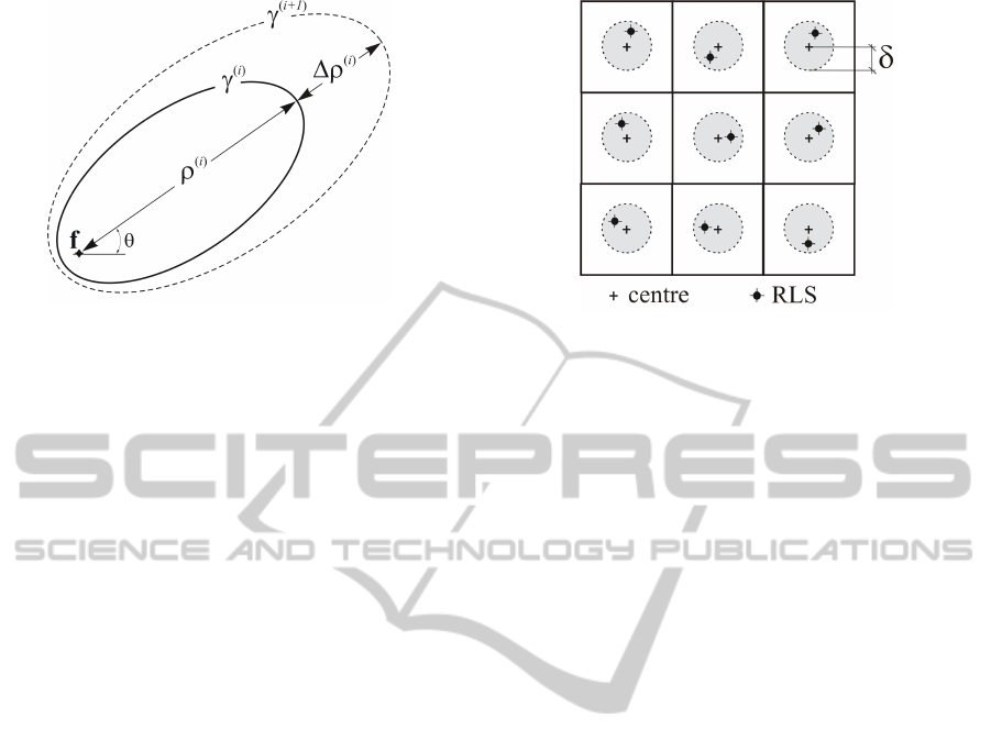
Figure 1: Growth of the ellipse γ locally representing the
fire front. The symbol ρ denotes the forward spread which
is incremented by ∆ρ at the i-th time step.
– Q is a set of random local sources (RLSs), one
point for each cell; they are randomly generated at
the beginning of the simulation within an assigned
radius δ from each of the centres in K , as shown
in Figure 2. As detailed later, a new ignition in a
cell consists of a new ellipse having its rear focus
on the local source q ∈ Q ;
– N is the set that identifies the pattern of cells in-
fluencing the cell state change (i.e the neighbour-
hood);
– S is the finite set of the states of the cell, defined
as the Cartesian product of the sets of definition
of all the cell’s substates;
– P is the finite set of global parameters which de-
fine the fuel bed characteristics according to the
standard fuel models used in BEHAVE (Andrews,
1986);
– ω : S
|N |
→ S is the transition function accounting
for the fire ignition, spread and extinction mecha-
nisms;
– Ψ is the set of global functions, activated at each
step before the application of the transition func-
tion ω to modify either the values of model param-
eters in P or the cells’ substates. Among these,
the function φ
τ
adapts the size p
∆t
of the time step
according to both the size of the cells p
e
and cur-
rent maximum spread rate in the whole automa-
ton. The value of p
∆t
is then used by another func-
tion, φ
t
, for keeping the current time up to date.
The cell’s substates include all the local quantities
used by the transition function for modelling the inter-
actions between cells (i.e. fire propagation to neigh-
bouring cells) as well as its internal dynamics (i.e. fire
ignition and growth). In particular, the relevant com-
ponents of the state of each cell are:
– the altitude z ∈ R;
Figure 2: An example of RLSs arrangement in a subset
of the automaton. Each RLS occupies a random position
within a distance δ from the cell centre.
– the fuel model µ ∈ N, which is an index referring
to one of the mentioned fuel models that spec-
ifies the characteristics of vegetation relevant to
Rothermel’s equations;
– the combustion state σ ∈ S
σ
, which takes one of
the values unburnable, not ignited, ignited and
burnt.
– the accumulated forward spread ρ ∈ R
≥0
, that is
the current distance between the focus f of the lo-
cal ellipse and the farthest point on the semi-major
axis (see Figure 1);
– the angle θ ∈ R (see Figure 1), giving the direc-
tion of the maximum rate of spread. In the con-
text of the semi-empirical Rothermel’s approach,
such an angle is obtained through the composition
of two vectors, namely the so-called wind effect
and slope effect (Rothermel, 1972), both obtained
on the basis of the local wind vector, local terrain
slope and fuel model;
– the maximum rate of spread r ∈ R
≥0
, also pro-
vided by Rothermel’s equations on the basis of the
relevant local characteristics (Rothermel, 1972);
– the eccentricity ε ∈ [0, 1] of the ellipse γ represent-
ing the local fire front, which is obtained as a func-
tion of both the wind and terrain slope through the
empirical relation proposed in (Anderson, 1983).
Among the remaining substates are the local wind
vector and the relative humidity value of the cell, both
provided as external input to the model.
As mentioned above, the CA model is based on
an extended Moore’s neighbourhood composed of 24
cells. Also, as explained below and represented in
Figure 2, the use of RLSs inside each cell allows for
obtaining a high number of different spread direction
during the fire propagation in the landscape, thus sig-
nificantly improving the accuracy of the results.
SIMULTECH2012-2ndInternationalConferenceonSimulationandModelingMethodologies,Technologiesand
Applications
262
The transition function ω concerns only cells that
are in the burning state. The first step of ω consists
of checking the condition that triggers the transition
to the burnt state. The latter is verified when all the
neighbouring cells are in either the ignited or in the
unburnable state, that is when the cell’s contribution
is no longer necessary to the fire spread mechanism.
Then, if the cell still belongs to the fire front, ω
updates the size of the local ellipse γ. This is accom-
plished by adding to the accumulated forward spread
ρ the product of the rate of spread r and the step size
∆t. The latter is dynamically established by the global
function φ
τ
according to the procedure proposed by
(Peterson et al., 2009).
The next step of ω consists of testing if the fire is
spreading towards other cells c
i
of the neighbourhood
that are in the not ignited state. Since in the current
cell the fire front is represented by a local ellipse γ,
such a spread test is carried out through checking if γ
includes the RLS q
i
of the cell c
i
(see Figure 3). To
this purpose the current spread in direction q
i
can be
easily computed using the mathematical properties of
the ellipse.
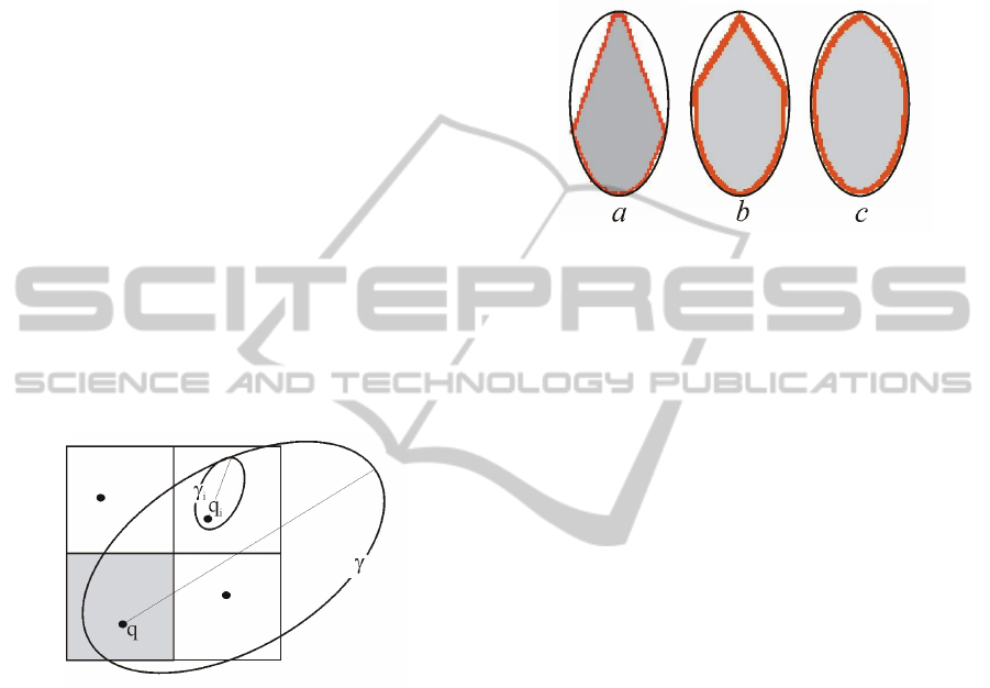
Figure 3: The i-th neighbouring cell intersected by the el-
lipse γ locally representing the fire front.
If q
i
is inside γ, then a new ellipse γ
i
is generated
for the cell c
i
, having the following characteristics:
• both the intensity r
i
of the maximum spread rate
vector and its inclination θ
i
are computed through
the proper Rothermel’s equations (Rothermel,
1972);
• the eccentricity ε
i
is determined using the empiri-
cal formula proposed by (Anderson, 1983), which
accounts for both the effect of wind and topog-
raphy through the previously mentioned effective
wind speed (McAlpine et al., 1991).
• as shown in Figure 3, its size is initialized so that
its most advanced point lies on the ellipse γ;
• the RLS q
i
is assumed as rear focus.
When compared with a typical CA algorithm for
wildfire simulation, the main advantage of the ap-
proach based on the RLSs, lies in its ability to in-
crease the directions of spread. This leads to an im-
proved accuracy as shown in Figure 4, where the ex-
pected fire shape under homogeneous conditions is
compared with the simulated shapes given by differ-
ent CA approaches.
Figure 4: A comparison between the simulated fire shapes
obtained under homogeneous condition with different CA
approaches: a) standard CA based on the Moore’s neigh-
bourhood and on a centre-to-centre ignition scheme; b) CA
based on an extended neighbourhood composed of 24 cells
with a centre-to-centre ignition scheme; c) CA based on the
same neighbourhood used in b) together with the RLSs. The
continuous line represents the expected shape.
2.2 A Simulation-based Approach for
Building BPMs
In the latest years, the use of hazard maps based on
the explicit simulation of natural phenomena has been
increasingly investigated as an effective and reliable
tool for supporting risk management (Rongo et al.,
2008; Carmel et al., 2009; Ager and Finney, 2009;
Rongo et al., 2011).
In the case of wildfire, the most general approach
for computing a BPM on a landscape (Carmel et al.,
2009; Ager and Finney, 2009) consists of a Monte
Carlo approach in which a high number of different
fire spread simulations are carried out, sampling from
suitable statistical distributions the random variables
relevant to the fire behaviour. For example, the wind
direction for each simulated fire can be sampled in a
range corresponding to the typical directions of severe
wind for the area. At the end of the process, the lo-
cal risk is computed on the basis of the frequency of
burning.
The technique for computing the BPMs adopted
in this study is based on a prefixed number n of
simulation runs, where each run represents a single
simulated fire. The adopted weather scenario (i.e.
wind and fuel moisture content) corresponds to ex-
treme conditions for the area with regards to relevant
historical fires. A regular grid of ignition locations
is adopted, which corresponds to the assumption of
a uniform ignition probability for each point of the
FastAssessmentofWildfireSpatialHazardwithGPGPU
263

landscape. Also, all the simulated fires have the same
duration. The latter is selected considering the du-
ration of historical fires in the regions under study.
All the other relevant characteristics are kept constant
during the simulations.
Once the latter have been carried out, the resulting
n maps of burned areas are overlaid and cells’ fire fre-
quency are used for the computation of the fire risk.
In particular, a burn probability p
b
(c) for each cell c
is computed as:
p
b
(c) =
f (c)
n
; (2)
where f (c) is the number of times the cell c is ignited
during the n simulated fires. The burn probability for
a given cell is an estimate of the likelihood that a cell
will burn given a single random ignition within the
study area and given the assumed conditions in terms
of fire duration fuel moisture and weather.
According to the procedure described above, the
number n of simulation runs depend on the resolution
of the grid of ignition points. In general, it is not nec-
essary to simulate a wildfire for each of the cells in
the automaton. In fact, considering the usual resolu-
tion of landscape data, ignitions on adjacent cells pro-
duce very similar fire shapes. Nevertheless, as shown
in the application example discussed later, the number
of fire simulation needed for achieving a good BPM
accuracy can be considerably high in case of study
areas with great extensions.
3 PARALLEL COMPUTING
WITH GPGPU
A natural approach to deal with the high computa-
tional effort related to construction of the BPMs, is the
use of parallel computing. Among the different paral-
lel architectures and computational paradigms, in the
last years GPGPU has attracted the interest of many
researchers (Preis, 2011; Roberts et al., 2010; Szer-
winski and G
¨
uneysu, 2008; Filippone et al., 2011;
Pallipuram et al., 2011; Krger et al., 2010). This is
mainly due to the following reasons:
• the computational power of devices enabling
GPGPU has exceeded that of standard CPUs by
more than one order of magnitude;
• the price of a typical device for GPGPU is com-
parable to the price of a standard CPU;
• there has been a rapid increase in the programma-
bility of these devices, which has facilitated the
porting of many scientific applications leading to
relevant parallel speedups (Krger et al., 2010).
Modern GPUs are multiprocessors with a highly ef-
ficient hardware-coded multi-threading support. The
key capability of a GPU unit is thus to execute thou-
sands of threads running the same function concur-
rently on different data (Single Instruction Multiple
Data archiecture). Hence, the computational power
provided by such an architecture, which can easily
reach a teraFLOP, can be fully exploited through a
fine grained data-parallel approach when the same
computation can be independently carried out on dif-
ferent elements of a dataset.
The particular GPGPU platform investigated in
this paper is the one provided by nVidia, which con-
sist of a group of Streaming Multiprocessors (SMs) in
a single device. Each SM can support a limited num-
ber of co-resident concurrent threads, which share the
SM’s limited memory resources. Furthermore, each
SM consists of multiple Scalar Processor (SP) cores.
In order to program the GPU, in this paper we
use the C-language Compute Unified Device Archi-
tecture (CUDA), a programming model introduced in
2006 by nVidia Corporation for their GPUs (NVidia
corp., 2010). In a typical CUDA program, sequential
host instructions are combined with parallel GPGPU
code. The idea underlying this approach is that the
CPU organizes the computation (e.g. in terms of
data pre-processing), sends the data from the com-
puter main memory to the GPU global memory and
invokes the parallel computation on the GPU device.
After, and/or during the computation, the computed
results are copied into the main memory for post-
processing and output purposes. In some cases, the
computing scheme outlined above can be enhanced
including overlapping the CPU and GPU computation
as well as overlapping memory copying with compu-
tation (NVidia corp., 2010; NVidia corp., 2012).
In CUDA, the GPGPU activation is obtained by
writing device functions in C language, which are
called kernels. When a kernel is invoked by the CPU,
a number of threads (e.g. typically several thou-
sands) execute the kernel code in parallel on differ-
ent data. From the kernel code it is possible to dis-
tinguish the currently associated thread through some
built-in variables (i.e. threadIdx, blockIdx, and block-
Dim). This allows to select from the device mem-
ory the data to associate to that particular thread (e.g.
the cell of a CA). According to the nVidia approach
to GPGPU, threads are grouped into blocks and exe-
cuted on a SMs.
From a programmer’s point of view, it is of a cer-
tain relevance to know that the GPU can access differ-
ent types of memory. For example, a certain amount
of fast shared memory (which can be used for some
limited intra-block communication between threads)
SIMULTECH2012-2ndInternationalConferenceonSimulationandModelingMethodologies,Technologiesand
Applications
264

can be assigned to each thread block. Also, all threads
can access a slower but larger global memory which
is on the device board but outside the computing chip.
The device global memory is slower if compared with
the shared memory, but it can deliver significantly
(e.g. one order of magnitude) higher memory band-
width than traditional host memory (i.e. the main
computer memory). The latter is typically linked to
the GPU card through a relatively slow bus. For ex-
ample, in most hardware configurations accessing the
host memory from the GPU can be more that 20 times
slower in terms of bandwidth (i.e. Gb/s) than access-
ing the global memory. As a result, the parallel com-
putation should be organised in such a way to mini-
mize data transfers between the host and the device.
For example, in some cases it is preferable to execute
on the device code which is inefficient (e.g. because
that specific part of the whole computation does not fit
well with the GPGPU model of parallelism) instead
of running it on the CPU, if this allows to avoid large
amount of CPU-GPU data transfers.
4 GPGPU-BASED WILDFIRE
RISK ASSESSMENT
The CA approach is known as one of the most typical
parallel computation paradigm. In fact, the whole sys-
tem is composed of a set of independent cells, which
are influenced only by their neighbours. This allows
for: (i) computing the next state of all the cells in
parallel; (ii) accessing only the current neighbours’
states during each cell’s update, thereby giving the
chance to increase the overall efficiency and making
easier even the implementation on distributed mem-
ory machines. As in the sequential case, the typical
CA parallel implementation involves two memory re-
gions representing the current and next states for the
cell. For each CA step, the neighbouring values from
current are read by the transition function, which per-
forms its computation and writes the new state value
into the appropriate element of next.
In particular, the GPGPU parallel implementa-
tion of the CA illustrated above, accordingly to the
recent literature in the field (Preis, 2011; Roberts
et al., 2010; Szerwinski and G
¨
uneysu, 2008; Filip-
pone et al., 2011), was based on the following design
choices:
• one or more CUDA computational kernels (i.e.
threads) are assigned to each cell of the automaton
as in (Filippone et al., 2011);
• most of the automaton data (i.e. both the cur-
rent and next memory areas mentioned above)
is stored in the GPU global memory. This in-
volves: (i) initialising the current state through
a CPU-GPU memory copy operation (i.e. from
host to device global memory) before the begin-
ning of the simulation and (ii) retrieving the final
state of the automaton at the end of the simulation
through a GPU-CPU copy operation (i.e. from de-
vice global memory to host memory). Also, at the
end of each CA step a device-to-device memory
copy operation is used to re-initialise the current
values with the next values.
In order to speed up the access to memory, the au-
tomaton data in device global memory should be or-
ganised in a way to allow coalescing access. To this
purpose, a best practice recommended by nVidia is to
use of structures of arrays rather than arrays of struc-
tures in organising the memory storage of cell’s prop-
erties (NVidia corp., 2012). Thus, while the typical
sequential implementation of the CA model described
in section 2 is based on structures or objects encapsu-
lating all the cells substates, in the GPGPU implemen-
tation it was more convenient to use simple arrays to
store the automaton. In particular, an array with the
size corresponding to the total number of cells was
allocated in the CPU memory for each of the CA sub-
states. All of such arrays were then mirrored in the
GPU together with some additional auxiliary arrays
(e.g. for storing the neighbourhood structure and the
model parameters).
A key step in the parallelisation of a sequential
code for the GPU architecture according to the CUDA
approach, consists of identifying all the sets of in-
structions that can be executed independently of each
other on different elements of a dataset (e.g., on the
different cells of the automaton). As mentioned in
Section 3, such sequences of instructions are grouped
in CUDA kernels, each transparently executed in par-
allel by the GPU threads. In particular, in the CA
model for wildfire simulation outlined in section 2,
two CUDA kernels have been developed:
• the kernel implementing the fire propagation
mechanism (i.e. the CA transition function ω);
• the kernel for dynamically adapting the time-step
duration. Since this involves finding the minimum
of all allowed time-step sizes among the cells on
the current fire front, such kernel simply imple-
ments a standard parallel reduction algorithm.
One of the critical aspects of the GPGPU imple-
mentation is related to the fact that in the whole au-
tomaton only the cells on the current fire front do ac-
tual computation in the transition function. Hence,
launching one thread for each of the automaton cells
results in a certain amount of dissipation of the GPU
FastAssessmentofWildfireSpatialHazardwithGPGPU
265

computational power. For this reason, besides the
standard CA implementation (SCA) in which the
above mentioned kernels are applied to each cells of
the automaton, a more optimized CA (OCA) has also
been developed. In the OCA, the kernel that adapts
the time-step size at each iteration, also computes
the smallest rectangular bounding box (RBB) that in-
cludes any cells on the current fire front, as shown
in Figure 5. Thus, the kernels implementing the CA
step are mapped only on such RBB, in this way re-
ducing the number of kernel launches and improving
significantly the computational performance of the al-
gorithm. It is worth noting that the same strategy has
been developed for the sequential version of the pro-
gram in order to obtain a fair comparison.
Figure 5: An example of the RBB representing the envelope
of the current fire front. In the OCA version, the CUDA
kernels are mapped only on the RBB.
However, notwithstanding the OCA approach,
during the simulation of a single fire the RBB still
includes a number of inactive cells. For example, all
the burned cells inside the current fire front are typi-
cally included in the RBB though they are not com-
putationally active. For this reason, in both the SCA
and OCA version of the algorithm, more than a sin-
gle fire are simultaneously simulated. In other words,
the above mentioned kernels iterate over a number of
active fires which are propagated simultaneously. Ob-
viously, such an approach requires the use of an inde-
pendent array for storing the combustion state σ of
each cell of the automaton and for each simultaneous
fire. At the cost of this additional memory occupa-
tion, the approach allows for increasing the level of
device saturation with beneficial effects on the com-
puting time.
Before starting the BPM construction, a pre-
processing sequential phase takes place in which for
each cell c
i
the maximum rate of spread r
i
, its direc-
tion θ
i
and the local ellipse eccentricity ε
i
(see Fig-
ure 1) are computed using the proper model equations
(Rothermel, 1972; Anderson, 1983). According to the
algorithm outlined in section 2, such pre-computed
quantities determine, together with the landscape to-
pography, the wildfire spread at the cell-level. Also,
during the pre-processing phase the maximum time-
step size for each cell is computed and stored in an ar-
ray in order to speed-up the time-step adaptation dur-
ing the CA iterations.
The process for the BPM computation is orga-
nized as follows. Cluster of fires are iteratively simu-
lated, up to covering the entire area under study (i.e.
up to the required number n of fires). In order to max-
imize the advantages of the OAC approach described
above, each cluster is composed of a block of contigu-
ous fires taken from the regular grid of fire ignitions.
For each cluster of simultaneous fires, the CA steps
are iterated until the current time p
t
reaches the final
time. In the parallel implementation, each CA step es-
sentially consists of the two CUDA kernels mentioned
above plus the device-to-device memory copy opera-
tion to re-initialise the current values of the substates
with the next values.
At the end of each group of simulations, a further
CUDA kernel is launched on the whole automaton to
update an array f
n
in which each element represents
the number of times that a cell has been burned since
the beginning of the process. As soon as all the sched-
uled simulations have been carried out, each element
of the array f
n
, divided by the total number of simu-
lations, gives an estimate of the burn probability for
one of the cells.
5 RESULTS ON A REAL
LANDSCAPE
The preliminary application presented here concerns
an area of the Ligury region, in Italy, historically
characterized by a high frequency of serious wild-
fires. The landscape, shown in Figure 6 was mod-
elled through a Digital Elevation Model composed of
461 × 445 square cells with side of 40 m. In the area,
the terrain is relatively complex with an altitude above
sea level ranging from 0 to 250 m. The heterogeneous
fuel bed depicted in Figure 6, was based on the use of
the 1:25000 land cover map from the CORINE EU-
project. The CORINE land-cover codes were mapped
on the standard fuel models used by the CA (i.e., the
substate µ). Plausible values of fuel moisture content
were obtained from literature data. Also, a domain-
averaged open-wind vector from the North direction,
having an intensity of 20 kmh
−1
, was used for produc-
ing time-constant gridded winds through WindNinja
(Forthofer et al., 2009), a computer program that sim-
ulates the effect of terrain on the wind flow. A du-
SIMULTECH2012-2ndInternationalConferenceonSimulationandModelingMethodologies,Technologiesand
Applications
266

Figure 6: The landscape under study: a 18km × 18km area in Ligury, Italy. Colors refer to the standard CORINE land-cover
data.
ration of 10 hours was adopted for all simulated fires.
Over the area, a regular grid of 91 ×88 ignition points
was superimposed, leading to 8008 fires to simulate.
Two CUDA graphic devices were used in the ex-
periments: a nVidia high-end Tesla C1060 and a
nVidia Geforce GT430 graphic card. In Table 1 some
of the relevant characteristics of the used GPGPU
devices are reported. The sequential programs, im-
plementing the same algorithms parallelised for the
GPGPU version, were run on a desktop computer
equipped with a 2.66 Ghz Intel Core 2 Quad CPU.
The two different implementations SCA and OCA de-
scribed in Section 4 were run on both the CPU and
GPU devices. In both cases, during the computation
process, 196 wildfires at a time were activated in or-
der to attain a satisfactory level of saturation of the
graphic device (see section 4).
The hazard map obtained after the n = 8008 sim-
ulations is shown in Figure 7. As shown in Table 2,
using the CPU the task took about 2.37 h for the SCA
version and about 1.44 h for the OCA implementa-
tion. As it can be seen in the same Table 2, the gain
provided by the parallelisation in terms of comput-
ing time is significant. In particular, through the most
powerful GPGPU the BPM computation took only 5
minutes using the SCA implementation and about 3.5
Table 1: Characteristics of the adopted GPGPU hardware
for all carried out experiments.
GT430 Tesla C1060
Compute capability 2.1 1.3
CUDA cores 96 240
Global memory [MB] 1024 4096
Clock rate [MHz] 1400 1300
Bandwidth [GB/s] 28.8 102.4
GFLOPs 268.8 922.12
Table 2: Elapsed times (in seconds) for the computation of
the BPM shown in Figure 7.
SCA OCA
CPU 8518.2 5185.6
GT430 771.6 417.5
Tesla C1060 301.7 209.1
Table 3: Parallel speedup achieved with the used GPGPU
devices.
SCA OCA
GT430 11.0 12.4
Tesla C1060 28.2 24.8
minutes using the OCA. Interestingly, even by using
the consumer-level GPGPU GT430, the computation
took only a few minutes.
According to Table 3, where the results in terms
of parallel speedups are shown, the highest speedup
of 28.2 was achieved by the Tesla C1060 using the
SCA approach. Overall, the results in terms of time
savings are significant, also considering the relatively
little effort required to develop the parallel versions of
the BPM computation algorithms. As before, it is also
worth noting that the GT430 graphic card, which pro-
vided here a parallel speedup of more than 10, costs
less than 60 Euros at the time of this publication.
As GPUs are specialized for single-precision cal-
culations, comparison tests were eventually carried
out with the aim of verifying the precision of results
between CPU-based outputs and GPUs’ ones. Here,
results were satisfactory, since the areal extensions of
simulations resulted the same, except for few approxi-
mation errors, limited to the 4
th
significant digit place,
in a limited number of cells.
FastAssessmentofWildfireSpatialHazardwithGPGPU
267
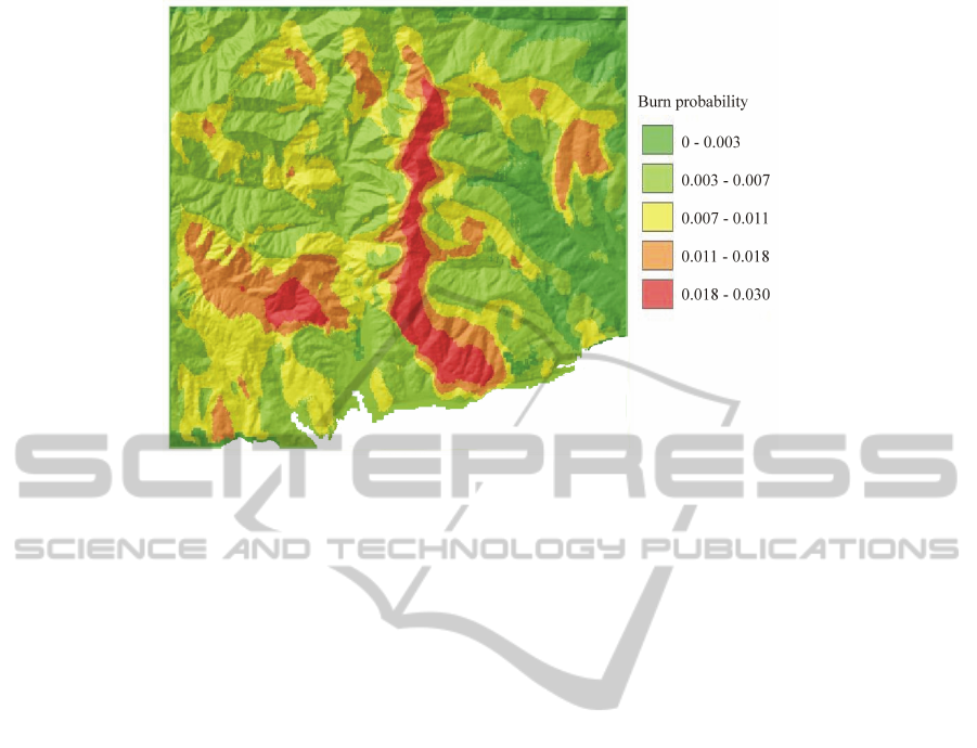
Figure 7: The BPM obtained for the landscape under study.
6 CONCLUSIONS AND FUTURE
WORK
The results in terms of parallel speedup of the
GPGPU-based BPM computation procedure pre-
sented above are indeed very encouraging. The main
advantage of such a parallelisation lies in enabling the
building of BPMs for large areas (e.g. at a regional
level), which otherwise may not be possible by adopt-
ing standard architectures.
Nevertheless, since not all the available GPGPU
optimization strategies have been implemented, am-
ple margins of speedup improvement are still pos-
sible. For example, since the only active cells are
the ones on the current fire front, even the OCA ap-
proach described above can permit to launch a sig-
nificant number of kernels on cells which are inac-
tive. A more advanced strategy could be used to map
mono-dimensional execution blocks only on the min-
imal number of cells lying on the fire front. An em-
pirical investigation will determine whether the com-
plexity related to the building of such complex grid
mapping would be compensated by the fewer kernels
to launch at each step of the automaton.
Another possible direction of research consists of
making available the GPGPU approach in more gen-
eral libraries for supporting CA modelling and sim-
ulation, such as the one presented in (Blecic et al.,
2009).
ACKNOWLEDGEMENTS
This work was partially funded by the European Com-
mission - European Social Fund (ESF) and by the Re-
gione Calabria (Italy).
REFERENCES
Ager, A. and Finney, M. (2009). Application of wildfire
simulation models for risk analysis. In Geophysical
Research Abstracts, Vol. 11, EGU2009-5489, EGU
General Assembly.
Alexander, M. (1985). Estimating the length-to-breadth ra-
tio of elliptical forest fire patterns. In Proc. 8th Conf.
Fire and Forest Meteorology, pages 287–304.
Anderson, H. (1983). Predicting wind-driven wildland fire
size and shape. Technical Report INT-305, U.S De-
partment of Agriculture, Forest Service.
Andrews, P. (1986). BEHAVE: fire behavior prediction and
fuel modeling system - burn subsystem, part 1. Tech-
nical Report INT-194, U.S Department of Agriculture,
Forest Service.
Blecic, I., Cecchini, A., and Trunfio, G. A. (2009). A
general-purpose geosimulation infrastructure for spa-
tial decision support. Transactions on Computational
Science, 6:200–218.
Carmel, Y., Paz, S., Jahashan, F., and Shoshany, M.
(2009). Assessing fire risk using monte carlo simula-
tions of fire spread. Forest Ecology and Management,
257(1):370 – 377.
Cui, W. and Perera, A. H. (2008). A study of simulation
errors caused by algorithms of forest fire growth mod-
els. Technical Report 167, Ontario Forest Research
Institute.
SIMULTECH2012-2ndInternationalConferenceonSimulationandModelingMethodologies,Technologiesand
Applications
268

Filippone, G., Spataro, W., Spingola, G., D’Ambrosio, D.,
Rongo, R., Perna, G., and Di Gregorio, S. (2011).
GPGPU programming and cellular automata: Imple-
mentation of the sciara lava flow simulation code. In
23rd European Modeling and simulation Symposium
(EMSS), Rome, Italy.
Forthofer, J., Shannon, K., and Butler, B. (2009). Simu-
lating diurnally driven slope winds with windninja. In
Proceedings of 8th Symposium on Fire and Forest Me-
teorological Society - Kalispell, MT.
French, I., Anderson, D., and Catchpole, E. (1990). Graphi-
cal simulation of bushfire spread. Mathematical Com-
puter Modelling, 13:67–71.
Johnston, P., Kelso, J., and Milne, G. (2008). Efficient sim-
ulation of wildfire spread on an irregular grid. Inter-
national Journal of Wildland Fire, 17:614–627.
Kourtz, P. H. and O’Regan, W. G. (1971). A model for a
small forest fire to simulate burned and burning ar-
eas for use in a detection model. Forest Science,
17(7):163–169.
Krger, F., Maitre, O., Jimenez, S., Baumes, L., and Collet, P.
(2010). Speedups between x70 and x120 for a generic
local search (memetic) algorithm on a single gpgpu
chip. In Di Chio, C., Cagnoni, S., Cotta, C., Ebner, M.,
Ek
´
art, A., Esparcia-Alcazar, A., Goh, C.-K., Merelo,
J., Neri, F., Preu, M., Togelius, J., and Yannakakis, G.,
editors, EvoNum 2010, volume 6024 of LNCS, pages
501–511. Springer Berlin / Heidelberg.
Lopes, A. M. G., Cruz, M. G., and Viegas, D. X. (2002).
Firestation - an integrated software system for the
numerical simulation of fire spread on complex to-
pography. Environmental Modelling and Software,
17(3):269–285.
McAlpine, R., Lawson, B., and Taylor, E. (1991). Fire
spread across a slope. In Proceedings of the 11th
Conference on Fire and Forest Meteorology (Society
of American Foresters: Bethesda, MD), pages 218–
225.
Miyamoto, H. and Sasaki, S. (1997). Simulating lava flows
by an improved cellular automata method. Computers
& Geosciences, 23(3):283–292.
NVidia corp. (2010). CUDA C Programming Guide v. 3.2.
NVidia corp. (2012). CUDA C Best Practices Guide.
O’Regan, W. G., Kourtz, P., and Nozaki, S. (1976). Bias
in the contagion analog to fire spread. Forest Science,
22.
Pallipuram, V., Bhuiyan, M., and Smith, M. (2011). A com-
parative study of GPU programming models and ar-
chitectures using neural networks. The Journal of Su-
percomputing, pages 1–46.
Peterson, S. H., Morais, M. E., Carlson, J. M., Denni-
son, P. E., Roberts, D. A., Moritz, M. A., and Weise,
D. R. (2009). Using HFIRE for spatial modeling of
fire in shrublands. Technical Report PSW-RP-259,
U.S. Department of Agriculture, Forest Service, Pa-
cific Southwest Research Station, Albany, CA.
Preis, T. (2011). GPU-computing in econophysics and sta-
tistical physics. The European Physical Journal - Spe-
cial Topics, 194(1):87–119.
Roberts, M., Sousa, M. C., and Mitchell, J. R. (2010). A
work-efficient gpu algorithm for level set segmenta-
tion. In ACM SIGGRAPH 2010 Posters, SIGGRAPH
’10, pages 53:1–53:1, New York, NY, USA. ACM.
Rongo, R., Lupiano, V., Avolio, M. V., D’Ambrosio, D.,
Spataro, W., and Trunfio, G. A. (2011). Cellular au-
tomata simulation of lava flows - applications to civil
defense and land use planning with a cellular automata
based methodology. In Kacprzyk, J., Pina, N., and
Filipe, J., editors, SIMULTECH 2011, pages 37–44.
SciTePress.
Rongo, R., Spataro, W., D’Ambrosio, D., Avolio, M. V.,
Trunfio, G. A., and Gregorio, S. D. (2008). Lava flow
hazard evaluation through cellular automata and ge-
netic algorithms: an application to mt etna volcano.
Fundam. Inform., 87(2):247–267.
Rothermel, R. C. (1972). A mathematical model for pre-
dicting fire spread in wildland fuels. Technical Re-
port INT-115, U.S. Department of Agriculture, Forest
Service, Intermountain Forest and Range Experiment
Station, Ogden, UT.
Rothermel, R. C. (1983). How to predict the spread and in-
tensity of forest and range fires. Technical Report INT-
143, U.S. Department of Agriculture, Forest Service,
Intermountain Forest and Range Experiment Station,
Ogden, UT.
Sullivan, A. (2009). Wildland surface fire spread mod-
elling, 1990-2007. 3: Simulation and mathematical
analogue models. International Journal of Wildland
Fire, 18:387–403.
Szerwinski, R. and G
¨
uneysu, T. (2008). Exploiting the
power of GPUs for asymmetric cryptography. In Pro-
ceedings of the 10th International Workshop on Cryp-
tographic Hardware and Embedded Systems (CHES
2008), pages 79–99, Washington, DC, USA.
Trunfio, G. A. (2004). Predicting wildfire spreading through
a hexagonal cellular automata model. In Sloot,
P. M. A., Chopard, B., and Hoekstra, A. G., edi-
tors, ACRI, volume 3305 of LNCS, pages 385–394.
Springer.
Trunfio, G. A., D’Ambrosio, D., Rongo, R., Spataro, W.,
and Gregorio, S. D. (2011). A new algorithm for simu-
lating wildfire spread through cellular automata. ACM
Trans. Model. Comput. Simul., 22(1):6.
Yassemi, S., Dragicevic, S., and Schmidt, M. (2008). De-
sign and implementation of an integrated GIS-based
cellular automata model to characterize forest fire be-
haviour. Ecological Modelling, 210(1-2):71–84.
FastAssessmentofWildfireSpatialHazardwithGPGPU
269
