
On the Design of Change-driven Data-flow Algorithms and Architectures
for High-speed Motion Analysis
Jose A. Boluda, Pedro Zuccarello, Fernando Pardo and Francisco Vegara
Departament d’Inform`atica, Escola T`ecnica Superior d’Enginyeria, Universitat de Val`encia,
Avda. de la Universidad, S/N. 46100 Burjassot, Valencia, Spain
Keywords:
High Speed Motion Analysis, Bioinspired Visual Sensing, Data-flow Architectures.
Abstract:
Motion analysis is a computationally demanding task due to the large amount of data involved as well as
the complexity of the implicated algorithms. In this position paper we present some ideas about data-flow
architectures for processing visual information. Selective Change Driven (SCD) is based on a CMOS sensor
which delivers, ordered by the absolute magnitude of its change, only the pixels that have changed after the
last time they were read-out. As a natural step, a processing architecture based on processing pixels in a data-
flow method, instead of processing complete frames, is presented. A data-flow FPGA-based architecture is
appointed in developing such concepts.
1 INTRODUCTION
Motion analysis is an important issue in the field of
computer vision, being the involved algorithms com-
monly based on the analysis of a sequence of still
images. This implies that most of the times there is
a large amount of data and the algorithms involved
are complex and time consuming. Researches have
focused their efforts onto improving the well-known
technology for acquiring images, or the computing
systems. Nevertheless, little effort has been put into
more innovative acquisition or computing approaches
to reduce this amount of calculus.
There are several different approaches for motion
analysis. From amongst them differential methods are
a type of motion analysis algorithm that typically in-
volves full image processing, where each image is a
snapshot taken at fixed intervals. Typically, the nor-
mal procedure implies the application of several pre-
processing filters on the entire image and for each im-
age in the sequence. Next, some more complex pro-
cessing stages are applied. Whether there have been
many changes in the image, only a few, or even no
changes at all. The sequence of instructions is sys-
tematically applied to the entire image. No matter if
there is any new relevant information, being a waste
of time and energy.
Visual systems of living beings can offer smarter
solutions in the topic of image processing. The visual
system of most biological systems does not capture
images and send them sequentially to the brain at a
fixed rate. The idea of a sequence of still snapshots
is not present in biological systems. Most biological
vision systems are based on different types of pho-
toreceptors that react to the light intensity delivering
its information asynchronously to higher levels of the
cognitive system (Gollisch and Meister, 2010).
A Selective Change Driven (SCD) camera deliv-
ers only the pixels that have changed since the last
read-out. A SCD sensor delivers only non-redundant
information, that is, information that has changed.
Moreover, pixel delivery is ordered by the absolute
magnitude of its change. Therefore, if there are time
constraints, the most significant changes in the im-
ages will be processed, discarding minor variations.
Following this argumentation, it is possible to imple-
ment a data-flow policy in the algorithm execution
with a conventional CPU, processing only those pix-
els that have changed. A pixel only triggers the in-
structions that depend on it. Moreover, it is possi-
ble to implement a custom data-flow architecture for
processing only changing information. This strategy
will decrease the total amount of data to be processed,
speeding-up the algorithm execution.
In the literature there have been other approaches
which go beyond the limitations of frame-grabber vi-
sion systems. In (Mahowald, 1992) it is proposed
the first silicon retina following Address-Event Rep-
resentation (AER) principles. Following this work,
many others have taken up the idea of replacing frame
548
Boluda J., Zuccarello P., Pardo F. and Vegara F..
On the Design of Change-driven Data-flow Algorithms and Architectures for High-speed Motion Analysis.
DOI: 10.5220/0004120805480553
In Proceedings of the 9th International Conference on Informatics in Control, Automation and Robotics (ICINCO-2012), pages 548-553
ISBN: 978-989-8565-21-1
Copyright
c
2012 SCITEPRESS (Science and Technology Publications, Lda.)

capturing, transmission and processing with single
pixel information (Higgins and Koch, 2000) (Chi
et al., 2007) (Lichtsteiner et al., 2008) (Camunas-
Mesa et al., 2010).
2 SCD SYSTEM AND
PROCESSING
A SCD system has as a main element a SCD camera,
and with this purpose, a new visual sensor which im-
plements the SCD behavior has been developed. The
sensor, built in CMOS technology, has a resolution
of 32x32 pixels and, although we assume this res-
olution is low for many applications, it is sufficient
for demonstration purposes and can even be useful in
some cases.
In the SCD sensor every pixel works indepen-
dently of the others. A capacitor is charged, simul-
taneously for each pixel, to a voltage during an inte-
gration time. Every pixel has an analogue memory
with the last read-out value. The absolute difference
between the current and the stored value is compared
for all pixels in the sensor; the pixel that differs most
is selected using a Winner-Take-All circuit (WTA)
(Zuccarello et al., 2010) and its illumination level and
coordinates are read out for processing. It is impor-
tant to note that the concept of snapshot at instant t
can be kept, taking into account that all the photodi-
ode charges begin and finish at the same time. The
subsequent read-out order is performed by the WTA
circuit. All the sensor control signals are generated
with a 32-bit PIC microcontroller running at 80 MHz
which is connected to a computer through a USB link.
Further details about this new sensor, the camera and
its use in limited-resources systems can be found in
(Pardo et al., 2011).
2.1 SCD Algorithms
The design of image processing algorithms within the
SCD formalism requires a change in the way of think-
ing about how the programming instructions are ap-
plied to data. A more detailed explanation of how
to develop SCD algorithms can be found in (Boluda
et al., 2011).
A generic motion analysis algorithm can, many
times, be modeled as a pipeline of successive differ-
ent transformations to the image flow: filtering, fea-
ture extraction, etc. Between these processing stages
intermediate values are stored. Most of them can be
understood as intermediate images, but others can not
be viewable in a straight forward way, these images
being called intermediate images. Thus, each stage of
the image processing pipeline (except the first which
has as input the initial pixel flow) has as input full in-
termediate images and also produces full intermediate
images as output. No matter whether or not the initial
pixels or intermediates results have changed. All the
instructions at each stage are inevitably applied to the
data, even if they do not generate any change.
The SCD execution flow is related with data-flow
architectures: each new pixel fires all the instructions
related with this new data. If there are no data changes
no instructions are fired (and neither time nor energy
is consumed). Initially the SCD camera delivers those
pixels that have changed (gray level and coordinates).
Then the first stage updates the contribution of this
new pixel value to its output intermediate images.
Following this idea all the stages do the same. When
new input data arrives at any intermediate stage, then
all the related instructions are fired, updating the out-
put intermediate images.
The SCD sensor, as already mentioned, allows a
special way of ´non-accurate
´
functioning. As the pix-
els are read-out by the magnitude of their change, it
could be possible not to process all the changing pix-
els, but only the first received pixels, which are those
that offer a greater variation. This behavior could be
desirable if there were computational time restrictions
and less accurate algorithm results could be accept-
able. Some experiments were been performed follow-
ing these ideas, simulating a SCD camera and apply-
ing this strategy to differential algorithms.
2.1.1 Linear Spatial Operators
Linear spatial operators are very common transfor-
mations used for preprocessing or feature extraction.
Spatial operators can be expressed as the systematic
application of a convolution mask to all the pixels of
the image. Let’s say that G is the result image of ap-
plying the M × M convolution mask w
i, j
to the image
I taken at instant t, then each G
x,y
pixel can be calcu-
lated as:
G
x,y
=
M−1
2
∑
i=
1−M
2
M−1
2
∑
j=
1−M
2
w
i, j
I
x+i,y+ j
(1)
where I
x,y
is a pixel of the image I.
With a SCD sensor, the way of computing the fil-
tered image G is different. There will be a set of n
′
changing pixels that have been taken at the same time,
not a full input image. The G image must be changed
only with the contributionof the n
′
pixels. An individ-
ual I
x,y
pixel taken at instantt+1 contributesto M×M
pixels of G, thus this input must be updated adding the
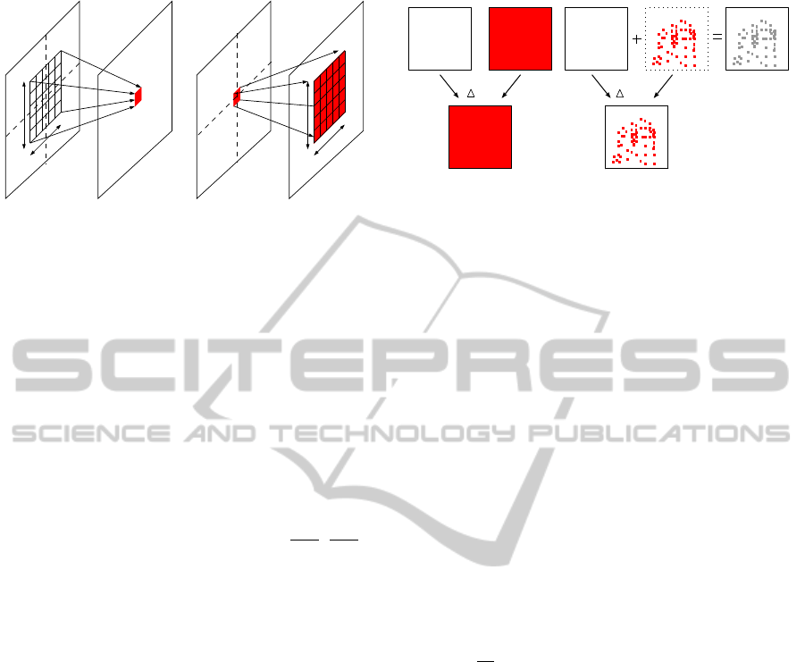
new value and removing the old one. Figure 1 shows
OntheDesignofChange-drivenData-flowAlgorithmsandArchitecturesforHigh-speedMotionAnalysis
549
M
M
y
x
Input
image I
Convolution
image G
(a) Classical spatial filtering
M
M
y
x
image I
Input
image G
Convolution
(b) SCD spatial filtering
Figure 1: Pixels involved in the computation of linear spa-
tial filtering.
an example of the application differences of a con-
volution mask in the classical way (a) and the SCD
method (b). It seems that there is a growing number
of operations, but it must be noted that the number
of operations remains constant if all the pixels have
changed. As this scenario is the worst case, in general
there will be much less operations. In general, when
the SCD camera delivers the pixel I
x,y
in the instant
t + 1 the modified pixels in the G image are:
G
x+i,y+ j
= G
x+i,y+ j
+w
−i,− j
(I
x,y
(t+1)−I
x,y
(t)) (2)
∀ i, j ∈
1−M
2
,
M− 1
2
The difference between the new I
x,y
(t + 1) and the
old value I
x,y
(t) is performed as a first operation. Af-
terwards, there are updated M
2
pixels of G.
It is possible to see how changing pixels trigger
the instructions that have a dependency with them.
This is the way SCD processing works. Only the
needed operations will be executed and no redundant
computations will be performed. In the case of spa-
tial dependency it is necessary to keep these interme-
diate images and write the modification algorithms in
a data-flow manner.
2.1.2 Temporal Processing
The implementation of temporal operators is essen-
tial for extracting motion from a video sequence. In
a simple classical implementation of a first order dif-
ferentiation, at least two frames taken at different in-
stants are kept in memory, past and present images,
and an operator computes results taken into account
both images. When a third new complete image is
taken then there is a shift between these images, the
past image being replaced by the present image (al-
ready in memory) and the present image is replaced
by the new acquired image, this one becoming the
new present image. No matter how many changed
pixels are in a new image. The temporal operators
I(t) I(t+1)
I(t)
I(t) I (t+1)
x,y
I (t)
x,y
I(t)
Figure 2: Comparison between the classical implementa-
tion of the differential operator and the SCD implementa-
tion.
are applied even if there are no new computations to
make. In the case of a pipelined hardware implemen-
tation, all the pixels of all the intermediate images
stored as input for computing a derivative stage, must
be replaced.
Within a SCD camera the system works in a differ-
ent way. Now there are no more full-frame incoming
images. Afterwards, only a set of changing pixels (ac-
quired at the same time) are read out. Because these
pixels have been taken at the same time the concept
of instant can be kept and transformation to the SCD
formalism is relatively straight forward.
As an example, let I(t) be the past image and
I(t + 1) the present image in the video sequence. In
the classical approach, a temporal derivative can be
approached in the simplest way as the subtraction be-
tween both images, this operation being performed
for the n pixels in the image.
dI
dt
x,y
≈ ∆I
x,y
= I
x,y
(t + 1) − I
x,y
(t) (3)
Only the subtraction operation must be performed
for the n
′
read-out pixels, which are the changing pix-
els, in the SCD approach. Additionally, only the new
pixel I
x,y
(t + 1) must update the image I(t), replacing
the old value in the image. If this differentiation is
made with intermediate images the process is identi-
cal. A changing intermediate pixel triggers the updat-
ing in its temporal operator, the intermediate value be-
ing updated in the source image. More complex oper-
ators such as a second derivative can be discomposed
into simpler spatial and temporal derivatives. Figure
2 shows the comparison between the differential op-
eration using both the classical and the SCD methods.
In the case of a pipelined hardware implementation,
only the changing pixels of the intermediate images
stored as input for computing a derivative stage, must
be replaced.
Other functions, as are non-parametrictransforms,
are converted into the SCD formalism in the same
way. Each new pixel triggers the related operations,
ICINCO2012-9thInternationalConferenceonInformaticsinControl,AutomationandRobotics
550
taken into account its contribution into the result im-
age of each stage.
3 A SIMPLE MOTION
DETECTION ALGORITHM
A moving edges detection algorithm for showing the
SCD methodologyhas been implemented by software
(Boluda et al., 2011). The algorithm is very simple
and works only in structured scenarios. The idea of
this experiment was not to contribute to the motion
detection in terms of accuracy or robustness. The
main idea was just to show how the SCD approach can
accelerate an image processing algorithm. The algo-
rithm computes the mean velocity of a single object in
a scene by detecting its edges through a convolution
mask, and then calculating its temporal variation sub-
tracting them between two successive frames. If this
difference is greater than a certain threshold, depend-
ing on the scene, then this pixel is taken into account
as belonging to the object. Assuming a rigid object
with a translation movement, the velocity of the mov-
ing edges will coincide with the object velocity. Ve-
locity data (u, v) are available in this example when
the third image has been completely processed. Aft er
that, a new pair of velocity components will be avail-
able after each new image has been processed. The
response of the system for updating the value of the
(u, v) pair will be the acquisition time of a full image
plus its transmission time and the algorithm comput-
ing time for the whole image. No matter the number
of changes that have been produced in the image. All
the operations will be performed systematically for all
the pixels in the image.
3.1 Selective Change-Drive Software
Version
The SCD version of the algorithm described previ-
ously was written (by software) in a data-flow man-
ner, following the rules described in this section. In
this version the SCD camera acquires an image at in-
stant t and sends the triplet: gray level intensity I
x,y
,
together with its coordinates (x, y), of the changing
pixels. As an extreme case, if there is not any moving
object, there will not be any gray level change, and
thus there will not be any delivered pixel and the sys-
tem will not process anything. In the other extreme
case, if all the intensity values have changed, all the
pixels will be sent and processed, giving no advantage
in terms of reduction of computations. Nevertheless,
it is shown experimentally that even with a high ra-
0 5 10 15 20 25 30
0
5
10
15
20
25
30
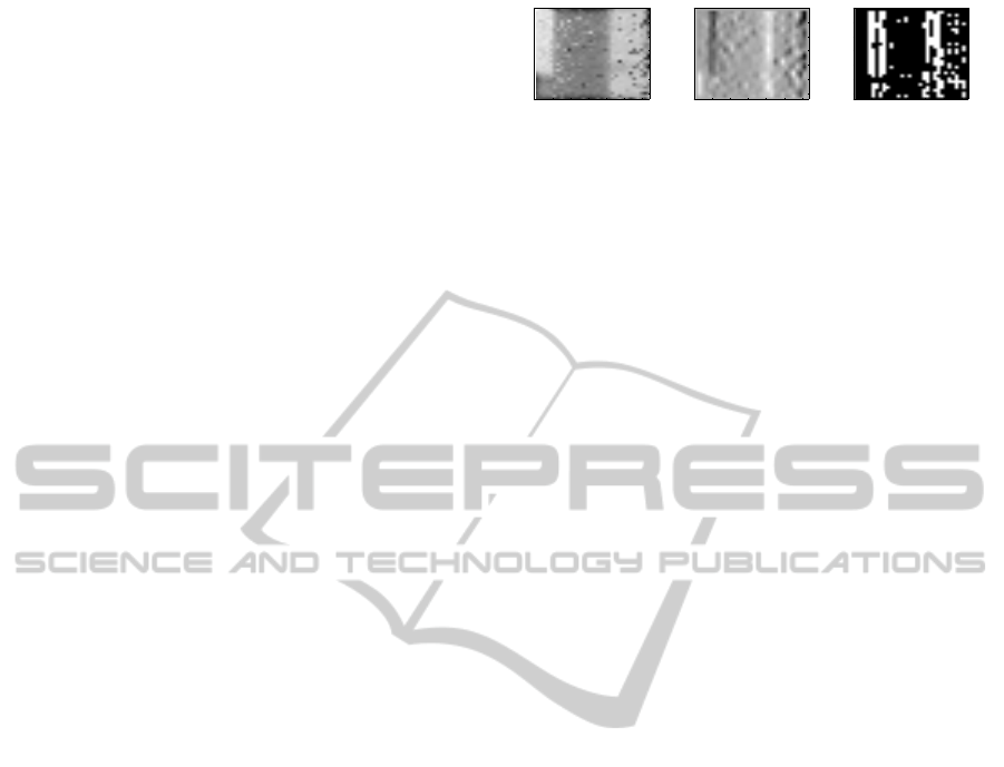
(a) SCD image
0 5 10 15 20 25 30
0
5
10
15
20
25
30
(b) Intermediate edges
image
0 5 10 15 20 25 30
0
5
10
15
20
25
30
(c) Bynarized edges dif-
ference image
Figure 3: Reconstructed images from the SCD data flow.
tio of changing pixels, a valuable speed-up with the
SCD system is achieved. Details about the SCD im-
plementation in terms of pseudo code can be found in
(Boluda et al., 2011).
3.2 Experimental Results
They have been performed several experiments with
32x32 pixel simulated images and with the real pixel
flow obtained from the SCD camera. First of all the
algorithm accuracy must be tested. That is, in a con-
trolled environment, and with images taken from a
conventional camera, the classical and the SCD algo-
rithm versions were tested. For the SCD version, the
data flow was simulated from a conventional camera,
giving exactly the same results both algorithms.
Following, the system was checked with the SCD
camera. Figure 3 shows several images from the per-
formed experiment. Inthis experiment, a vertical strip
was placed over a small vehicle moving horizontally
from right to left. The scene may appear simple, but
with a 32x32 sensor complexobjects are not recogniz-
able and simpler geometric forms are ideal for testing
purposes.
The image shown in Figure 3 (a) is the accumula-
tive image that has been reconstructed by adding the
changing pixels delivered by the SCD camera. The
image is noisy, since strategies for correcting the im-
age quality in CMOS imagers (fixed pattern noise,
etc.) have not been applied in order to show real im-
ages supplied by the SCD sensor. A simple Sobel fil-
ter for the x coordinate transformed to the SCD for-
malism has been applied, as shown in section 2.1.1, to
implement the filter stage. The image shown in Figure
3 (b) shows edges correctly detected as well as some
spurious small edges corresponding to noisy pixels.
Finally, Figure 3 (c) shows the bynarized edges differ-
ence image from the last stages of the SCD algorithm.
From successive difference images, the velocity com-
ponents (u, v) are obtained as the center of mass of
the moving edges. There is some accuracy loss in
the velocity data due to the presence of noisy pix-
els that are contributing to the position of the object.
Nevertheless, the reasons for this loss of accuracy, due
to the use of real images, will be corrected in further
versions of the camera firmware, applying image im-
OntheDesignofChange-drivenData-flowAlgorithmsandArchitecturesforHigh-speedMotionAnalysis
551
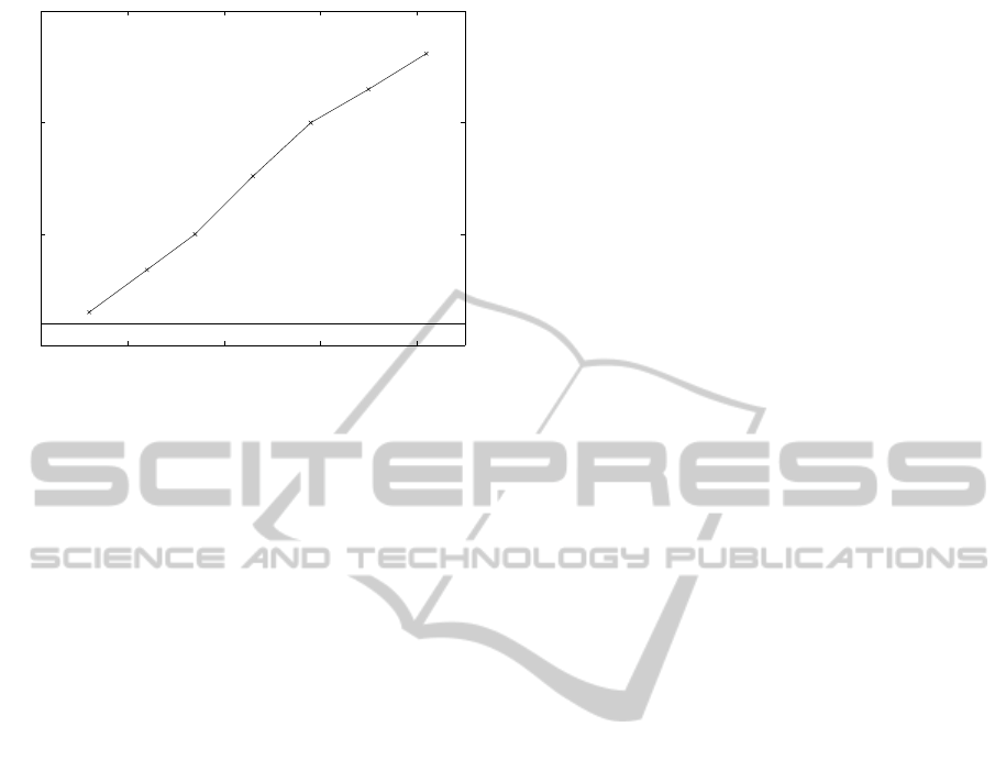
10 20 30 40
0
5
10
15
Number of SCD images
SCD algorithm speed−up
Figure 4: Speed-up execution time of the SCD algorithm
versus the original implementation.
proving strategies for CMOS visual sensors.
Figure 4 shows the speed-up obtained with the
performed experiment by software. Clearly, the
speed-up will depend of the number of changing pix-
els. With fewer changing pixels, less redundant oper-
ations will perform the SCD algorithm compared to
the classical version and the algorithm speed-up will
increase. In the moving edge sequence, there is an
average of roughly 50% of pixels that change. There-
fore, we can see that we do not need a low quantity
of changing pixels to obtain a valuable speed-up with
this strategy.
Figure 4 shows the achieved speed-up with the
SCD algorithm versus the classical version, in func-
tion of the number of frames. The speed-up increases
with the number of images due that there is a fixed
cost per image in the classical algorithm: compu-
tations are performed whether or not there are any
changing pixels and thus the related computations are
needed. This cost is always greater than the SCD al-
gorithm cost in each image. The speed-up asymp-
totically will approach the quotient between the cost
of both algorithms, original and SCD. This quotient
has been computed, giving a theoretical speed-up of
roughly 300. Therefore, Figure 4 really shows the ini-
tial part of an asymptote that, as the number of images
increases, approaches its speed-up to the ideal value
of 300. This speed-up depends on the experiment: ob-
jects velocity, illumination conditions, etc. A deeper
explanation and analysis of the moving-edge experi-
ment (in its software version) can be seen at (Boluda
et al., 2011).
4 HARDWARE VERSION
In this position paper we claim that the motion de-
tection algorithm in the SCD version can be im-
plemented into a data-flow architecture, and this is
our current work: to implement all this ideas into a
hardware-based platform. All the experiments per-
formed until now have been made by software achiev-
ing, nevertheless, a valuable speed-up.
It must be considered that the SCD formalism is
a special case of data-flow architectures, where each
incoming pixel change triggers the related operations.
Figure 5 shows a schema of the proposed pipelined
architecture, currently being developed into an AL-
TERA FPGA-based board. The pipeline has 5 stages,
having as input of the first stage the SCD pixel flow,
that is, the triplet formed by the grey level together
with their coordinates: (I, x, y). The output of the sys-
tem are the (u, v) velocity components.
The first stage just updates the SCD image with
the pixels coming from the SCD camera. The SCD
image is stored in a 32x32 array of 1-byte registers.
The second stage is fired when the new pixel replaces
the old one. This second stage computes the pixel
contribution of the new pixel to the convolution im-
age. The incoming pixel contributes to 8 pixels in the
convolution image following the equation 2, since the
chosen Sobel filter has a mask of 3x3 pixels.
Stage 3 stores changes into one of the two follow-
ing register banks. The update image at instant t has
information of the most important changes produced
at this instant, but also includes changes produced in
the past. Each time the camera acquires a new image,
the stage switches the storage bank. The older image
is replaced by the new one with the new pixels when
the updating of the newer frame has been finished.
Then the newer frame can be updated again with the
changes coming from the precedent stage.
Stage 4 reads the two frames and marks the corre-
sponding coordinate of a pixel pair (binarized image)
if the difference is greater than a certain threshold that
depends on the experiment. Stage 5 computes the
centre of mass of the contributing points and makes
the subtraction to the centre of mass of the preceding
image. The velocity components (u, v) are then deliv-
ered as the result of the algorithm.
5 CONCLUSIONS
In this position paper we propose a change-driven
processing architecture for image processing as an al-
ternative to full-frame processing systems. This al-
ternative will speed-up classical motion analysis al-
ICINCO2012-9thInternationalConferenceonInformaticsinControl,AutomationandRobotics
552
Stage 2
Convolution maskUpdate image
Stage 1 Stage 3
writing
Differential
Stage 4
Binarization
Stage 5
computation
Velocity
(I,x,y) (u,v)
SCD image
array of registers
Convolution
image image
Binarized
Image (t+1)
Image (t)
Figure 5: Data-flow pipeline.
gorithms since it reduces the total amount of com-
putations performed. The recently developed 32x32
CMOS sensor delivers the changing pixels from the
present frame to the last sent frame at each integra-
tion time. Several theoretical studies following this
strategy were presented in the past with real images
constructed from the original SCD data-flow. The
current paper presents some ideas for implementing
an already made SCD software implementation into a
FPGA-based platform.
There appear as a natural continuation to this ex-
periments performed by software, the principles of
data-flow processing and architectures. Within these
architectures a pixel fires the instructions that depend
on it, instead of following the imperative program-
ming model. The change-driven processing strategy
presented in this paper follows these ideas.
This kind of system is oriented to real-time image
processing, or systems that need very high speed pro-
cessing. The SCD strategy will deliver non-redundant
data, and the data-flow processing system will per-
form, precisely, the needed computations, with the
lowest latency possible. Further versions of the SCD
camera firmware, and further sensors with greater res-
olution, will provide the potential for the implementa-
tion of much more complex and accurate algorithms
that will operate at the highest possible speed.
ACKNOWLEDGEMENTS
This work has been supported by the Spanish Govern-
ment project TEC2009-12980.
REFERENCES
Boluda, J., Zuccarello, P., Pardo, F., and Vegara, F. (2011).
Selective Change Driven Imaging: A Biomimetic Vi-
sual Sending Strategy. Sensors, 11(11):1100–11020.
Camunas-Mesa, L., Perez-Carrasco, J., Zamarreno-Ramos,
C., Serrano-Gotarredona, T., and Linares-Barranco,
B. (2010). On Scalable Spiking ConvNet Hardware
for Cortex-Like Visual Sensory Processing System. In
Proc. of the 2010 IEEE International Symposium on
Circuits and Systems, pages 249–252, Paris, France. .
Chi, Y., Mallik, U., Clapp, E., Choi, E., Cauwenberghs,
G., and Etienne-Cummings, R. (2007). CMOS cam-
era with in-pixel temporal change detection and ADC.
IEEE Journal of Solid-State Circuits, 42(10):2187–
2196.
Gollisch, T. and Meister, M. (2010). Eye smarter than sci-
entist believed: Neural computations in circuits of the
Retina. Neuron, 65():150–164.
Higgins, C. and Koch, C. (2000). A Modular Multi-Chip
Neuromorphic Architecture for Real-Time Visual Mo-
tion Processing. Analog Integrated Circuits and Sig-
nal Processing, 24(3):195–211.
Lichtsteiner, P., Posch, C., and Delbr¨uck, T. (2008). A
128x128 dB 15 µs latency asynchronous temporal
contrast vision sensor,. IEEE Journal of Solid-State
Circuits, 43(2):566–576.
Mahowald, M. (1992). VLSI Analogs of neural visual pro-
cessing: A synthesis of form and function. PhD thesis,
Computer Science Divivision, California Institute of
Technology, Pasadena, CA.
Pardo, F., Zuccarello, P., Boluda, J., and Vegara, F. (2011).
Advantages of Selective Change Driven Vision for
resource-limited systems. IEEE Transactions on Cir-
cuits and Systems for Video Technology, 21(10):1415–
1423.
Zuccarello, P., Pardo, F., de la Plaza, A., and Boluda, J.
(2010). 32x32 winner-take-all matrix with single win-
ner selection. Electronics Letters, 46(5):333–335.
OntheDesignofChange-drivenData-flowAlgorithmsandArchitecturesforHigh-speedMotionAnalysis
553
