
Microwave Design Optimization Exploiting Adjoint Sensitivity
Slawomir Koziel, Leifur Leifsson and Stanislav Ogurtsov
Engineering Optimization & Modeling Center, School of Science and Engineering, Reykjavik University, Reykjavik, Iceland
Keywords: Computer-aided Design (CAD), Simulation-driven Design, Microwave Design Optimization,
Electromagnetic Simulation, Adjoint Sensitivity.
Abstract: Adjustment of geometry and material parameters is an important step in the design of microwave devices
and circuits. Nowadays, it is typically performed using high-fidelity electromagnetic (EM) simulations,
which might be a challenging and time consuming process because accurate EM simulations are
computationally expensive. In particular, design automation by employing an EM solver in an numerical
optimization algorithm may be prohibitive. Recently, adjoint sensitivity techniques become available in
commercial EM simulation software packages. This makes it possible to speed up the EM-driven design
optimization process either by utilizing the sensitivity information in conventional, gradient-based
algorithms or by combining it with surrogate-based approaches. In this paper, we review several recent
methods and algorithms for microwave design optimization using adjoint sensitivity. We discuss advantages
and disadvantages of these techniques and illustrate them through numerical examples.
1 INTRODUCTION
Contemporary microwave engineering heavily relies on
electromagnetic (EM) simulation. EM simulation is not
only used for design verification but in the design
process itself, i.e., to adjust geometry and/or material
parameters of the structure under consideration.
Unfortunately, accurate EM simulation is CPU
intensive. A way to speed it up is parallelization
(OpenMP, MPI, GPU) or distributed computing.
However, the bottleneck in EM-simulation-based
optimization remains to be the large number of EM
simulations required by conventional optimization
algorithms. Another problem is related to the numerical
noise present in EM-based objective functions, due to
which local search methods often fail to find the
optimal design. While many commercial EM
simulation packages have implemented basic design
automation methods (mostly conventional gradient-
based and derivative-free approaches such as Quasi-
Newton or Nelder-Mead algorithms, or population-
based algorithms such as genetic algorithms), a
common practice is still to obtain satisfactory design
using tedious and time-consuming parameter sweeps
involving numerous full-wave EM simulations
combined with engineering experience.
Efficient simulation-driven design can be
performed using surrogate based optimization
(SBO). The most successful SBO techniques in
microwave engineering include space mapping (SM)
(Bandler et al., 2004); (Koziel et al., 2008a); (Amari
et al., 2006), simulation-based tuning (Swanson and
Macchiarella, 2007); (Rautio, 2008), manifold
mapping (MM) (Echeverria and Hemker, 2005), as
well as shape-preserving response prediction
(Koziel, 2010). While the SBO techniques can be
extremely efficient, they are not straightforward to
automate to make them reliable “push-button”-like
approaches that could work for a variety of
microwave problems. Their use typically requires
some experience (Koziel et al., 2008a) and most of
them are not globally convergent so that whether a
satisfactory design is obtained or not may depend on
a proper implementation, some parameter tuning, as
well as certain knowledge particularly while
constructing the surrogate model.
Another approach to improve efficiency of
simulation-driven design is by using adjoint sensitivity
that allows obtaining derivative information of the
system of interest with little or no extra computational
cost (Nair and Webb, 2003); (El Sabbagh et al., 2006);
(Kiziltas et al., 2003); (Uchida et al., 2009); (Bakr et
al., 2011). However, until recently, adjoint sensitivities
were not commercially available, which means that
they were not available for most engineers and
designers. Situation changed a few years ago when
499
Koziel S., Leifsson L. and Ogurtsov S..
Microwave Design Optimization Exploiting Adjoint Sensitivity.
DOI: 10.5220/0004164104990506
In Proceedings of the 2nd International Conference on Simulation and Modeling Methodologies, Technologies and Applications (SDDOM-2012), pages
499-506
ISBN: 978-989-8565-20-4
Copyright
c
2012 SCITEPRESS (Science and Technology Publications, Lda.)

adjoint sensitivities were implemented for instance in
CST Microwave Studio (CST, 2011).
In this paper, we review several recent
techniques that exploit adjoint sensivity in order to
speed up the EM-simulation-driven microwave
design process. These techniques include gradient-
based search methods embedded in trust region
framework, as well as surrogate-based methods,
specifically space mapping (Koziel et al., 2008a) and
manifold mapping (Echeverria and Hemker, 2005),
enhanced by adjoint sensitivity in order to improve
their convergence properties and reduce the
computational cost of surrogate model optimization
step. The efficiency of the presented approaches is
demonstrated using several microwave design cases.
A performance comparison with other optimization
techniques, including Matlab’s fminimax (Matlab,
2008) and a Quasi-Newton type of algorithm
(Nocedal and Wright, 2000) is also provided.
2 DESIGN OPTIMIZATION WITH
TRUST-REGION AND ADJOINT
SENSITIVITIES
2.1 Design Problem Formulation
The microwave design task can be formulated as a
nonlinear minimization problem
*
argmin ( )
ff
U
x
x R x
(1)
where R
f
R
m
denotes the response vector of a high-
fidelity (or fine) model of the microwave structure
of interest evaluated through expensive high-fidelity
EM simulation; x R
n
is a vector of designable
variables. Typically, these are geometry and/or
material parameters. The response R
f
(x) might be,
e.g., the modulus of the transmission coefficient |S
21
|
evaluated at m different frequencies. In some cases,
R
f
may consists of several vectors representing, e.g.,
filter reflection and transmission coefficients, or an
antenna reflection, gain, etc. U is a given scalar
merit function, e.g., a norm, or a minimax function
with upper and lower specifications. U is formulated
so that a better design corresponds to a smaller value
of U. x
f
*
is the optimal design to be determined.
Direct solution of (1) using conventional
algorithm may be prohibitive because it usually
requires a large number of fine model evaluations,
each being computationally expensive by itself. For
many structures, the evaluation time may be as long
as a few hours.
2.2 Trust-Region-Based Optimization
with Adjoint Sensitivity
The algorithm proposed in (Koziel et al., 2012a)
uses the 1st-order model (or the surrogate) S(x) of
the high-fidelity model Rf. S(i)(x) is nothing else but
a linear function being a first-order Taylor expansion
of Rf at x(i) of the form:
( ) ( ) ( ) ( )
( ) ( ) ( )
( , , ( ), ( ))
( ) ( ) ( )
f
f
i i i i
f
i i i
f
J
J
R
R
S x x R x x
R x x x x
(2)
J
Rf
(x) is an estimated Jacobian of R
f
at x,
J
Rf
(x) = [∂R
fi
/∂x
j
]
i=1,…,m; j=1,…,n
, obtained using adjoint
sensitivity (if available) or finite differentiation
∂R
fi
/∂x
j
[R
fi
([x
1
… x
j
+d
j
… x
n
]
T
) – R
fi
(x)]/d
j
for all
the other parameters.
The optimization algorithm framework is the
following (r
0
is the initial trust region radius)
1. i = 0; r = r
0
;
2. Optimize a linear model: x
tmp
= argmin{||x – x
(i)
||
≤ r : S
(i)
(x,x
(i)
,R
f
(x
(i)
),J
F
(x
(i)
))};
3. Calculate gain ratio:
= [U(R
f
(x
(i)
) –
U(R
f
(x
tmp
))]/[U(R
f
(x
(i)
) – U(S(x
tmp
))];
4. If U(R
f
(x
tmp
)) < U(R
f
(x
(i)
)) then x
(i+1)
= x
tmp
;
i = i + 1;
5. Update r:
< r
decr
then r = r/m
decr
; else if
> r
incr
then r = r·m
incr
;
6. If termination condition is not satisfied, go to 2;
else, END.
Here, r
decr
and r
incr
denote threshold values for
decreasing or increasing the trust region radius by
the corresponding factors m
decr
and m
incr
. The
algorithm is terminated if either of the following
conditions is satisfied: r <
r
, n
F
< n
Fmax
, ||x
(i)
– x
(i–1)
||
<
x
, or ||U(R
f
(x
(i)
)) – U(R
f
(x
(i–1)
))|| <
F
, where
r
,
x
,
F
, n
Fmax
, are user defined parameters, whereas n
F
is
the number of high-fidelity model evaluations.
The response Jacobian is recalculated after each
successful iteration (i.e., when U(R
f
(x
tmp
)) <
U(R
f
(x
(i)
))) for those variables where adjoint
sensitivity is available. The finite-difference
sensitivity is not recalculated as long as the new
iteration is successful in order to reduce the number
of high fidelity function evaluations.
The above algorithm is a local-search method.
Assuming that the exact sensitivity of Rf at x(i) is
used to define the first-order model S(i), S(i)
satisfies both zero- and first-order consistency
conditions with the high-fidelity model Rf, i.e.,
S(i)(x(i)) = Rf(x(i)) and JS(x(i)) = JRf(x(i)). This is
sufficient for the global convergence of the
SIMULTECH 2012 - 2nd International Conference on Simulation and Modeling Methodologies, Technologies and
Applications
500

algorithm at least to a local optimum of the high-
fidelity model, provided that Rf is sufficiently
smooth (Alexandrov et al., 1998). In practice, the
high-fidelity model is noisy, nevertheless, the
performance of the algorithm is quite remarkable
(Koziel et al., 2012a).
Responses obtained using EM solvers are
inherently noisy (except, perhaps, when the mesh
topology is fixed). The major reason is that the mesh
topology is a discontinuous function of the design
variables (or, more general, of geometry of the
structure under considerations). The minor reason is
that the evaluation process itself is noisy (e.g., due to
finite tolerances used to terminate the EM
simulation). This poses some problems for the
optimization process. In particular, finite
differentiation with conventional small increments
(e.g., 10
–8
) will not work: the value of the derivative
obtained this way will be completely unreliable,
regardless of the model discretization density. The
reason is that the change of the response due to the
small perturbation of any given design variable will
be, most likely, much smaller than the amplitude of
the numerical noise. For noisy functions, better and
more consistent gradient estimation can be obtained
using larger finite differentiation step sizes. Based
on the above considerations, our algorithm uses
relatively large steps for finite differentiation,
typically, 10
–3
or larger (depending on the absolute
values of the design variables).
2.3 Example: Design of a Waveguide
Bandpass Filter
Consider the waveguide filter shown in Fig. 1.
Design variables are [h
1
h
2
h
3
s
1
s
2
s
3
s
4
w
1
w
2
w
3
w
4
]
T
. Design specifications are |S
11
| –20 dB for
667.5 MHz
675 MHz. The initial design is x
(0)
= [163.5 172 165.3 160.5 160.5 160.5 130.5 –60.5 –
29.5 –28.5 –27.5]
T
(minimax specification error
+19.2 dB). Optimization results are shown in Table
1. Figure 2 shows the filter responses at the initial
design and at the optimized design found by the
algorithm of Section 2.2. In this case, the proposed
algorithm performs substantially better than the
methods used for comparison both with respect to
the computational cost of the design process and the
quality of the final design. It should be noted that the
computational complexity of our algorithm using
finite-differences derivatives is comparable to that of
Matlab’s fminimax, even though the latter exploits
adjoint sensitivity.
3 SURROGATE-BASED
OPTIMIZATION WITH
ADJOINT SENSITIVITY
3.1 Surrogate-based Optimization
A generic surrogate-based optimization (SBO)
algorithm (Koziel and Yang, 2011); (Forrester and
Keane, 2009) generates a sequence of approximate
solutions to (1), x
(i)
, as follows
( 1) ( )
argmin ( )
ii
s
U
x
x R x
(3)
Figure 1: Geometry of a waveguide bandpass filter.
(a)
(b)
Figure 2: Waveguide bandpass filter: (a) responses at the
initial design x
(0)
; (b) responses at the optimized design
found by the proposed algorithm using mixed adjoint and
finite-difference sensitivities.
660 665 670 675 680 685
-30
-20
-10
0
Frequency [MHz]
|S
11
|
660 665 670 675 680 685
-30
-20
-10
0
Frequency [MHz]
|S
11
|
Microwave Design Optimization Exploiting Adjoint Sensitivity
501

Table 1: Optimization results for the waveguide bandpass
filter.
Optimization Algorithm
Final
Specification
Error
Number of
Function
Evaluations
Quasi-Newton optimizer
+5.3 dB
1454
Matlab’s fminimax
+1.2 dB
88
This work
(Algorithm of
Section 2)
Adjoint sensitivity
–2.2 dB
16
Mixed adjoint /
finite-difference
sensitivity
*
–1.3 dB
46
Finite-difference
sensitivity
–0.4 dB
107
* Adjoint sensitivity for the first seven variables, finite-
differences for the remaining four variables.
where R
s
(i)
is the surrogate model at iteration i. Here,
x
(0)
is the initial design. R
s
(i)
is assumed to be a
computationally cheap and sufficiently reliable
representation of R
f
, particularly in the neighborhood
of x
(i)
. Under these assumptions, the algorithm (3) is
likely to produce a sequence of designs that quickly
approach x
f
*
. Usually, R
f
is only evaluated once per
iteration (at every new design x
(i+1)
) for verification
purposes and to obtain the data necessary to update
the surrogate model. Because of the low
computational cost of the surrogate model, its
optimization cost can usually be neglected and the
total optimization cost is determined by the
evaluation of R
f
. The key point here is that the
number of evaluations of R
f
for a well performing
surrogate-based algorithm is substantially smaller
than for most conventional optimization methods.
3.2 Robustness of SBO Algorithms
Robustness of the surrogate-based optimization
process (3) depends on the quality of the surrogate
model R
s
(i)
. In general, in order to ensure
convergence of the algorithm (3) to at least local
optimum of the high-fidelity model, the first-order
consistency conditions have to be met (Alexandrov
and Lewis, 2001), i.e., one has to have R
s
(i)
(x
(i)
) =
R
f
(x
(i)
) and J
R
s
(i)
(x
(i)
) = J
R
f
(x
(i)
), where J stands for the
Jacobian of the respective model. Also, the process (3)
has to be embedded in the trust-region (TR)
framework (Conn et al., 2000), i.e., we have
( ) ( )
( 1) ( )
:|| ||
arg min ( ( ))
ii
ii
s
U
x x x
x R x
(4)
where the TR radius
(i)
is updated using classical
rules (Conn et al., 2000). In general, the SBO
algorithm (4) can be successfully utilized without
satisfying the aforementioned conditions, see, e.g.
(Bandler et al., 2004); (Koziel et al., 2008a).
However, in these cases, the quality of the
underlying low-fidelity model may be critical for
performance (including the algorithm convergence)
(Koziel et al., 2008b) and accurate location of the
optimum design may not be possible.
Availability of cheap adjoint sensitivity (Nair
and Webb, 2003); (CST, 2011) makes it possible to
satisfy consistency conditions in a easy way (without
excessive computational cost by using, e.g., finite
differentiation). A few options exploiting this
possibility are discussed in the next section.
3.3 SBO with First-order Taylor Model
and Trust Regions
The simplest way of exploring adjoint sensitivity for
antenna optimization is to use the following
surrogate model for the SBO scheme (4):
( ) ( ) ( ) ( )
( ) ( ) ( ) ( )
f
i i i i
sf
R
R x R x J x x x
(5)
where J
Rf
is the Jacobian of R
f
obtained using
adjoint sensitivity technique. The key point of the
algorithm is finding the new design x
(i)
and the
updating process for the search radius
(i)
. Here,
instead of the standard rules, we use the following
strategy (x
(i–1)
and
(i–1)
are the previous design and
the search radius, respectively):
1. For
k
= k
(i–1)
, k = 0, 1, 2, solve:
()
()
:|| ||
arg min ( ( ))
i
k
ki
s
U
x x x
x R x
. Note that x
0
= x
(i–1)
. The
values of
k
and U
k
= U(R
s
(i)
(x
k
)) are interpolated
using 2
nd
-order polynomial to find
*
that gives the
smallest (estimated) value of the specification error
(
*
is limited to 3
(i–1)
). Set
(i)
=
*
.
2. Find a new design x
(i)
by solving (4) with the
current
(i)
.
3. Calculate the gain ratio
= [U(R
f
(x
(i)
)) – U
0
]/
[U(R
s
(i)
(x
(i)
)) – U
0
]; If
< 0.25 then
(i)
=
(i)
/3; else
if
> 0.75 then
(i)
= 2
(i)
;
4. If
< 0 go to 2;
5. Return x
(i)
and
(i)
;
The trial points x
k
are used to find the best value of
the search radius, which is further updated based on
the gain ratio
(actual versus expected objective
function improvement). If the new design is worse
than the previous one, the search radius is reduced to
find x
(i)
again, which eventually will bring the
improvement of U as R
s
(i)
and R
f
are first-order
SIMULTECH 2012 - 2nd International Conference on Simulation and Modeling Methodologies, Technologies and
Applications
502

consistent (Alexandrov and Lewis, 2001). This
precaution is necessary because the procedure in
Step 1 only gives an estimation of the search radius.
As an example, consider a wideband hybrid
antenna (Petosa, 2007) shown in Fig. 3, a quarter-
wavelength monopole loaded by dielectric ring
resonator. The design goal is to have |S
11
| ≤ −20 dB
for 8-to-13 GHz. The design variables are x = [h
1
h
2
r
1
r
2
g]
T
. The initial design is x
(0)
= [2.5 9.4 2.3 3.0
0.5]
T
mm. Other parameters are fixed. The final
design with the proposed algorithm is x
(0)
= [3.94
10.01 2.23 3.68 0.0]
T
mm. Table 2 and Fig. 4
compare the design cost and quality of the final
design found by the algorithm described above and
Matlab’s fminimax. It can be observed that our
algorithm yields better design at significantly
smaller computational cost (75 percent design time
reduction).
3.4 Space Mapping and Manifold
Mapping
Construction of the surrogate model can also be
based on the underlying low-fidelity (or coarse)
model R
c
, e.g., obtained from coarse-discretization
EM simulation data. The two methods considered
here that use this approach are space mapping (SM)
(Koziel et al., 2008a) and manifold mapping (MM)
(Echeverria and Hemker, 2005). Usually, the
knowledge about the system embedded in the low-
fidelity model allows us to reduce the number of
high-fidelity model evaluations necessary to find an
optimum design.
The SM surrogate considered here is constructed
using input and output SM (Bandler et al., 2004) of
the form:
( ) ( ) ( ) ( ) ( )
( ) ( ) ( )
i i i i i
sc
R x R x c d E x x
(6)
Here, only the input SM vector c
(i)
is obtained
through the nonlinear parameter extraction process
( ) ( ) ( )
argmin|| ( ) ( )||
i i i
fc
c
c R x R x c
(7)
Output SM parameters are calculated as
( ) ( ) ( ) ( )
( ) ( )
i i i i
fc
d R x R x c
(8)
and
( ) ( ) ( ) ( )
( ) ( )
fc
i i i i
RR
E J x J x c
(9)
Formulation (6)-(9) ensures zero- and first-order
consistency (Alexandrov and Lewis, 2001) between the
surrogate and the fine model.
The manifold mapping (MM) surrogate model is
defined as (Echeverria and Hemker, 2005)
( ) ( ) ( ) ( )
( ) ( ) ( ) ( )
i i i i
s f c c
R x R x S R x R x
(10)
where S
(i)
is the mm correction matrix defined as
( ) ( ) ( ) †
( ) ( )
fc
i i i
RR
S J x J x
(11)
Figure 3: Wideband hybrid antenna: geometry.
Figure 4: Wideband hybrid antenna: reflection response at
the initial design ( ), at the final design by Matlab’s
fminimax (- - -), and by the proposed algorithm (—).
Table 2: Wideband hybrid antenna: design results.
Algorithm
max|S
11
| for 8 to 13 GHz
at Final Design
Design Cost
(Number of EM
Analyses)
Matlab’s
fminimax
–22.6 dB
98
This work
–24.6 dB
24
The pseudoinverse, denoted by
†
, is defined as
††
c
c c c
T
R R R
R J J J
JVΣU
(12)
where U
J
Rc
,
J
Rc
, and V
J
Rc
are the factors in the
singular value decomposition of J
R
c
. The matrix
J
Rc
†
is the result of inverting the nonzero entries in
J
Rc
, leaving the zeroes invariant (Echeverria and
Hemker, 2005). Using the sensitivity data as in (12)
h
2
h
1
g
GND
50 Ω coax
r
1
r
2
ε
1
ε
2
ε
3
ε
1
ε
2
r
0
d
d
d
6 8 10 12 14 16
-35
-30
-25
-20
-15
-10
-5
0
Frequency [GHz]
|S
11
| [dB]
Microwave Design Optimization Exploiting Adjoint Sensitivity
503

ensures that the surrogate model (10) is first-order
consistent with the fine model. In our
implementation, the coarse model is preconditioned
using input space mapping of the form (7) in order
to improve its initial alignment with the fine model.
Both the parameter extraction (7) and surrogate
model optimization processes (4) are implemented
by exploiting adjoint sensitivity data of the low-
fidelity model, which allows for further cost savings.
The details of these implementations can be found in
(Koziel et al., 2012b).
In order to illustrate the operation and
performance of the SM and MM algorithms, let us
consider an UWB antenna shown in Fig. 5. The
antenna and its models include: a microstrip
monopole, housing, edge mount SMA connector,
section of the feeding coax. The design variables are
x = [l
1
l
2
l
3
w
1
]
T
. Simulation time of the low-fidelity
model R
c
(156,000 mesh cells) is 1 min, and that of
the high-fidelity model R
f
(1,992,060 mesh cells) is
40 min (both at the initial design). Both models are
simulated with the transient solver of CST
Microwave Studio (CST, 2011). The design
specifications for reflection are |S
11
|
≤
–12 dB for 3.1
GHz to 10.6 GHz. The initial design is x
init
= [20 2 0
25]
T
mm.
The antenna was optimized using the SBO
algorithm (4) with both the SM and MM surrogate
models. Fig. 6(a) shows the responses of R
f
and R
c
at
x
init
. Fig. 6(b) shows the response of the high-fidelity
model at the final design x
(2)
= [20.22 2.43 0.128
19.48]
T
(|S
11
|
≤
–12.5 dB for 3.1 to 10.6 GHz) obtained
after only two SBO iterations with MM surrogate, i.e.
only 4 evaluations of the high-fidelity model (Table
3). The number of function evaluations is larger than
the number of MM iterations because some designs
can be rejected by the TR mechanism. The algorithm
using SM surrogate required three iterations and the
final design is x
(3)
= [20.29 2.27 0.058 19.63]
T
(|S
11
|
≤
–12.8 dB for 3.1 to 10.6 GHz) obtained after three
SM iterations. The total optimization cost (Table 4) is
equivalent to around 6 evaluations of the fine model.
Figure 7 shows the evolution of the specification
algorithm for the manifold mapping algorithm.
As another example, consider the third-order
Chebyshev bandpass filter (Kuo et al., 2003) shown in
Fig. 8. The design variables are x = [L
1
L
2
S
1
S
2
]
T
mm.
Other parameters are: W
1
= W
2
= 0.4 mm. Both fine
(396,550 mesh cells, evaluation time 45 min) and
coarse (82,350 mesh cells, evaluation time 1 min)
models are evaluated by the CST MWS transient solver
(CST, 2011).
The design specifications are |S
21
| –3 dB for
1.8 GHz
2.2 GHz, and |S
21
| –20 dB
for
1.0
GHz
1.55GHz and 2.45 GHz
3.0 GHz. The
initial design is the coarse model optimal solution
x
init
= [16 16 1 1]
T
mm.
(a)
(b)
Figure 5: UWB monopole: (a) 3D view; (b) top view. The
housing is shown transparent.
(a)
(b)
Figure 6: UWB monopole optimized using manifold
mapping algorithm: (a) responses of R
f
(—) and R
c
(- - -)
at the initial design x
init
; (b) response of R
f
(—) at the
final design.
The filter was optimized using the SM algorithm.
Optimization results are shown in Fig. 9 and Table
5. The final design x
(5)
= [14.58 14.57 0.93 0.56]
T
is
obtained after five SM iterations. As before,
optimization cost is very low. Also, thanks to
sensitivity information as well as trust region, the
algorithm improves the specification error at each
iteration, see Fig. 10. This is not the case for
GND
l
1
l
2
l
3
w
1
2 4 6 8 10 12
-20
-15
-10
-5
Frequency [GHz]
|S
11
| [dB]
2 4 6 8 10 12
-20
-15
-10
-5
Frequency [GHz]
|S
11
| [dB]
SIMULTECH 2012 - 2nd International Conference on Simulation and Modeling Methodologies, Technologies and
Applications
504
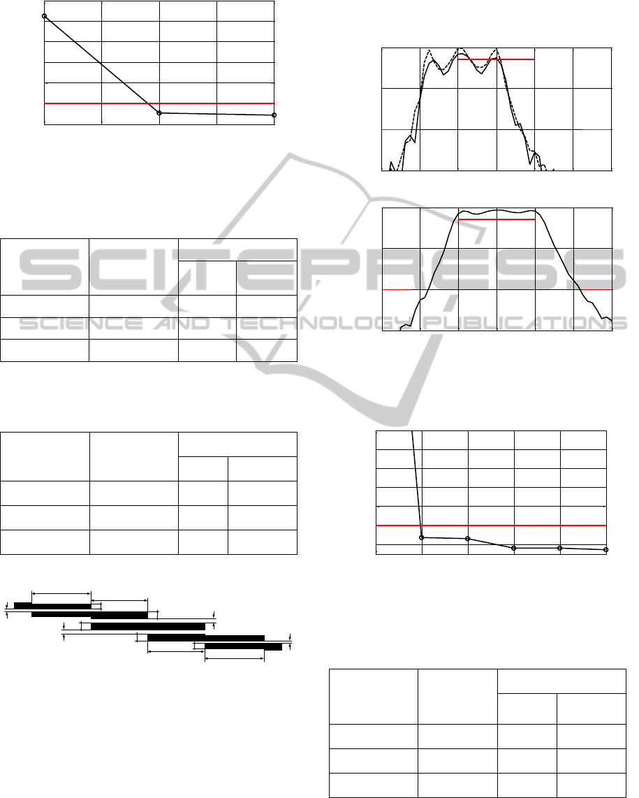
conventional space mapping (Bandler et al., 2004).
Figure 7: UWB monopole: Minimax specification error
versus manifold mapping algorithm iteration index.
Table 3: UWB monopole antenna: optimization results
using manifold mapping.
Algorithm
Component
Number of Model
Evaluations
*
CPU Time
Absolute
Relative to
R
f
Evaluation of R
c
31
31 min
0.8
Evaluation of R
f
4
120 min
4.0
Total cost
*
N/A
151 min
4.8
* Includes R
f
evaluation at the initial design.
Table 4: UWB monopole antenna: optimization results
using space mapping.
Algorithm
Component
Number of Model
Evaluations
*
CPU Time
Absolute
Relative to R
f
Evaluation of R
c
45
45 min
1.1
Evaluation of R
f
5
200 min
5.0
Total cost
*
N/A
205 min
6.1
* Includes R
f
evaluation at the initial design.
Figure 8: Third-order Chebyshev bandpass filter: geometry.
4 CONCLUSIONS
A review of recent microwave design optimization
techniques exploiting adjoint sensitivity has been
presented. We have demonstrated that by exploiting
cheap derivative information, the EM-simulation-
driven design process can be performed efficiently
and in a robust way. Adjoint sensitivity can also be
used to improve performance of the surrogate-based
optimization algorithm as illustrated on the example
of space mapping and manifold mapping techniques.
(a)
(b)
Figure 9: Third-order Chebyshev filter: (a) responses of R
f
(—) and R
c
(- - -) at the initial design x
init
; (b) response of
R
f
(—) at the final design.
Figure 10: Third-order Chebyshev filter: minimax
specification error versus SM iteration index.
Table 5: Third-order Chebyshev filter: optimization
results using space mapping.
Algorithm
Component
Number of
Model
Evaluations
*
CPU Time
Absolute
Relative to R
f
Evaluation of R
c
67
67 min
1.5
Evaluation of R
f
6
270 min
6.0
Total cost
*
N/A
337 min
7.5
* Includes R
f
evaluation at the initial design.
0 0.5 1 1.5 2
-1
0
1
2
3
4
5
Iteration index
Specification error [dB]
L
1
W
1
S
1
L
2
L
1
L
2
S
2
S
2
S
1
W
2
W
2
W
1
W
2
1.4 1.6 1.8 2 2.2 2.4 2.6
-30
-20
-10
0
Frequency [GHz]
|S
21
| [dB]
1.4 1.6 1.8 2 2.2 2.4 2.6
-30
-20
-10
0
Frequency [GHz]
|S
21
| [dB]
0 1 2 3 4 5
-1
0
1
2
3
4
5
Iteration index
Specification error [dB]
Microwave Design Optimization Exploiting Adjoint Sensitivity
505

ACKNOWLEDGEMENTS
The authors would like to thank CST AG for making
CST Microwave Studio available. This work was
supported in part by the Icelandic Centre for
Research (RANNIS) Grant 110034021.
REFERENCES
Alexandrov, N. M., Dennis, J. E., Lewis, R. M., Torczon,
V., 1998. A trust region framework for managing use
of approximation models in optimization. Struct.
Multidisciplinary Optim., vol. 15, no. 1, pp. 16-23.
Alexandrov, N. M., Lewis, R. M., 2001, An overview of
first-order model management for engineering
optimization. Optimization Eng., vol. 2, no. 4, pp. 413-
430.
Amari, S., LeDrew, C., Menzel, W., 2006. Space-mapping
optimization of planar coupled-resonator microwave
filters. IEEE Trans. Microwave Theory Tech., vol. 54,
no. 5, pp. 2153-2159.
Bakr, M. H., Ghassemi, M., Sangary, N., 2011, Bandwidth
enhancement of narrow band antennas exploiting
adjoint-based geometry evolution. IEEE Int. Symp.
Antennas Prop., pp. 2909-2911.
Bandler, J. W., Cheng, Q. S., Dakroury, S. A., Mohamed,
A. S., Bakr, M. H., Madsen, K., Søndergaard, J., 2004.
Space mapping: the state of the art. IEEE Trans.
Microwave Theory Tech., vol. 52, no. 1, pp. 337-361.
Conn, A. R., Gould, N. I. M., Toint, P. L., 2000. Trust
Region Methods, MPS-SIAM Series on Optimization.
CST MICROWAVE STUDIO®, 2011, CST AG, Bad
Nauheimer Str. 19, D-64289 Darmstadt, Germany.
El Sabbagh, M. A., Bakr, M. H., Nikolova, N. K., 2006,
Sensitivity analysis of the scattering parameters of
microwave filters using the adjoint network method.
Int. J. RF and Microwave Computer-Aided Eng., vol.
16, no. 6, pp. 596-606.
Echeverria, D., Hemker, P. W., 2005. Space mapping and
defect correction. CMAM The International
Mathematical Journal Computational Methods in
Applied Mathematics. vol. 5, no. 2, pp. 107-136.
Forrester, A. I .J., Keane, A. J., 2009. Recent advances in
surrogate-based optimization, Prog. in Aerospace
Sciences, vol. 45, no. 1-3, pp. 50-79.
Kiziltas, G., Psychoudakis, D., Volakis, J. L., Kikuchi, N.,
2003, Topology design optimization of dielectric
substrates for bandwidth improvement of a patch
antenna. IEEE Trans. Antennas Prop., vol. 51, no. 10,
pp. 2732-2743.
Koziel, S., Cheng, Q. S., Bandler, J. W., 2008a. Space
mapping. IEEE Microwave Magazine, vol. 9, no. 6,
pp. 105-122.
Koziel, S., Bandler, J. W., Madsen, K., 2008b, Quality
assessment of coarse models and surrogates for space
mapping optimization. Optimization and Engineering,
vol. 9, no. 4, pp. 375-391.
Koziel, S., 2010. Shape-preserving response prediction for
microwave design optimization. IEEE Trans.
Microwave Theory and Tech., vol. 58, no. 11, pp.
2829-2837.
Koziel, S., Yang, X. S., (Eds.), 2011, Computational
optimization, methods and algorithms, Series: Studies
in Computational Intelligence, vol. 356, Springer.
Koziel, S., Mosler, F., Reitzinger, S., Thoma, P., 2012a,
Robust microwave design optimization using adjoint
sensitivity and trust regions. Int. J. RF and Microwave
CAE, vol. 22, no. 1, pp. 10-19.
Koziel, S., Ogurtsov, S., Bandler, J. W., Cheng, Q. S.,
2012b, Robust space mapping optimization exploiting
EM-based models with adjoint sensitivity. IEEE MTT-
S Int. Microwave Symp. Dig.
Kuo, J. T., Chen, S. P., Jiang, M., 2003, Parallel-coupled
microstrip filters with over-coupled end stages for
suppression of spurious responses. IEEE Microwave
and Wireless Comp. Lett., vol. 13, no. 10, pp. 440-442.
Matlab, Version 7.6, 2008, The MathWorks, Inc., 3
Apple Hill Drive, Natick, MA 01760-2098.
Nair, D., Webb, J. P., 2003, Optimization of microwave
devices using 3-D finite elements and the design
sensitivity of the frequency response. IEEE Trans.
Magn., vol. 39, no. 3, pp. 1325-1328.
Nocedal, J., Wright, S. J., 2000, Numerical Optimization,
Springer Series in Operations Research, Springer.
Petosa, A., 2007. Dielectric Resonator Antenna
Handbook, Artech House.
Rautio, J. C., 2008. Perfectly calibrated internal ports in EM
analysis of planar circuits. IEEE MTT-S Int. Microwave
Symp. Dig., Atlanta, GA, pp. 1373-1376.
Swanson, D. Macchiarella, G., 2007, Microwave filter
design by synthesis and optimization. IEEE
Microwave Magazine, vol. 8, no. 2, pp. 55-69.
Uchida, N., Nishiwaki, S., Izui, K., Yoshimura, M.,
Nomura, T., Sato, K., 2009, Simultaneous shape and
topology optimization for the design of patch
antennas. European Conf. Antennas Prop., pp. 103 –
107.
SIMULTECH 2012 - 2nd International Conference on Simulation and Modeling Methodologies, Technologies and
Applications
506
