
Intelligent Predicting Method of Water Bloom based RBFNN
and LSSVM
Liu Zaiwen
1
, Wu Qiaowei
2
and Lv Siying
2
1
School of Computer and Information Engineering, Beijing Technology and Business University, Beijing 100048, China
2
Graduate School, Beijing Technology and Business University, Beijing 100048, China
Keywords: Predicting Method, Water Bloom, RBF Neural Network, Squares Support Vector Machine, Intelligence.
Abstract: Water bloom is one phenomena of eutrophication, and water bloom prediction is always a challenge. A
short-term intelligent predicting method based on RBF neural network (RBFNN), and medium-term
intelligent predicting method based on least squares support vector machine (LSSVM) for water bloom are
proposed in this paper. Including research on the monitoring learning algorithms to the center, width and
weight of basis function of RBF network, the width of RBF and fitting and generalization abilities of
network, and the function and influence, which the number of RBF hidden level nodes brings to the
performance of network, as well as error-corrected algorithm based on gradient descent are analyzed. Least
squares support machine, which has long prediction period and high degree of prediction accuracy, needs a
small amount of sample can be used to predict the medium-term change discipline of Chl-a (Chlorophyll-a)
well. The results of simulation and application show that: RBF neural network can be used to forecast the
change of Chl-a in short term well, and LSSVM improves the algorithm of support vector machine (SVM),
and it has long-term prediction period, strong generalization ability and high prediction accuracy; and this
model provides an efficient new way for medium-term water bloom prediction.
1 INTRODUCTION
Eutrophication is the result of pollutioroups of high
density in water body; and alga water bloom is one
phenomena of eutrophication which is caused by the
contamination of lakes, pools and reservoirs etc.
(Welch et al., 1986). Many eutrophication models
with different complicacy have been developed both
on theory and practice: from simple model with
single state variable, Vollenweider TP model to
complex ecosystem model with dynamic simulation.
These models are of great importance on research
and management of water eutrophication
(Somlyody, 1998); (Vollenweider, 1975)
.
At present, most methods are mainly based on the
change of influencing factors to predict water bloom.
Ecological numerical models are considered as the
trend of research and predicting of water bloom and
red tide (Guisen et al., 2005).
Support Vector Machine (SVM) can use kernel
function to solve the practical problems of small
amount of sample, nonlinearity, high dimension and
partial minimum point well. This model, which can
be successfully used in temporal series prediction
area, has become one of the most practical methods
of machine learning technology. Currently, in the
water bloom prediction research which has the
characteristics of temporal series, artificial neural
network is most frequently used. But trying to
research based on SVM will provide a new idea for
water bloom prediction methods (Qing, 2001); (Wu
et al., 2000).
2 A SHORT-TERM PREDICTING
METHOD BASED ON RBF
NEURAL NETWORK
2.1 Calculation by Radial Basis
Function (RBF) Neural Network
RBF is a forward neural network with two levels,
including a hidden layer with radial basis function
neuron and an output layer with linear neuron. The
center of RBF is calculated by monitoring learning
methods, which are also adopted to train the center,
weight and width of RBF. Error correction algorithm
592
Zaiwen L., Qiaowei W. and Siying L..
Intelligent Predicting Method of Water Bloom based RBFNN and LSSVM.
DOI: 10.5220/0004334705920597
In Proceedings of the 5th International Conference on Agents and Artificial Intelligence (ICAART-2013), pages 592-597
ISBN: 978-989-8565-39-6
Copyright
c
2013 SCITEPRESS (Science and Technology Publications, Lda.)

based on gradient descent is discussed as follows
(Van Gestel et al., 2004).
Object function is defined as:
2
1
1
2
N
j
j
E
e
(1)
1
() ( )
m
jj j j i ji
ci
i
edFx d wGxt
(2)
Where N is the number of samples, m is the
number of hidden units selected, there are three
parameters to be learned:
ji
w
,
i
t
and
1
i
(connected with changing matrix
i
C
The learning rules of error connection method
through gradient descent are shown as follows (n is
the number of iterating ).
1) the output of weight of unit:
1
()
() ( () )
()
N
jji
ci
j
i
En
enGx tn
wn
i=1,2,…,m
(3)
2) the center of hidden unit:
1
()
2() ()( ()
()
N
ij ji
ci
i
j
En
wn e nG x t n
tn
1
() ()
ji
i
nx tn
(4)
3) the width of function:
'
1
1
()
() () ( ()
()
N
ij ji
ci
j
i
En
wn e nG x t n
n
()
T
ji
x
tn
(5)
Where
'
G(g)is the differential coefficient of
Green function.The width of radial basis function is
fixed according to the fitting and generalization of
network.
2.2 Improve RBF Algorithm
If function
2
()
d
hLR
is radial, there will be a
function
2
L
. For
d
x
R
, there is a
formula
() ( )hx x
(6)
Where
x
is the range of x. According to
formula(9), the common expression of radial basis
function is:
1
() (( ) ( ))
T
hx x c E x c
(7)
Where Ф represents radial basis function,
c
represents central vector of function, E is
changing matrix.
The performance of RBF network mostly
depends on the center. RBF with linear parameters
can be outspread on the prediction that Ф(.) and
center C are fixed
[7-8]
. The common radial basis
functions include:
Gaussian Function:
22
(/ )
()
t
te
(8)
Multiquadric Function:
22
() 1/( )
a
tt
(
a
>0)
(9)
Gaussian Function is in most common use,
because of several reasons as follows:
● The form of function is simple, even to multi-
variable inputs.
● Radial symmetry, good smoothness, derivative
with any rank exists.
● Function is easy to analyze theoretically.
The design of hidden node keeps to smallest
network structure satisfying the precision, in order to
ensure the generalization of network.
2.3 Determination of Prediction Model
Parameters
A lot of indicate that the growth of phycophyta is
influenced by many kinds of factors. Among these
factors, the most important restricted factor is
nitrogen and phosphorus which are necessary
nutrient source for the growth of hydrophytes. Water
body chlorophyll concentration is an important
reference index for measure of water body primary
productivity and eutrophication situation and it is
also ultimate index of water body algae stock on
hand and judgment of water bloom.
Thus, Chl-a is used to be output variable of
prediction model. History data of Chl_a should also
be considered to be the input variable of prediction
model.
2.4 Predicting Model of Water Bloom
The first 56 groups of data interpolated in RBF are
chosen to be the training data, and the other 4 groups
of data are taken as test data. After that, a three-level
network with multi inputs and single output can be
established (Zaiwen Liu, 2009)
.
The parameters of soft sensing models are set as
follows:
5 Secondary variables: temperature (TW),
transparency (SD), electric conductivity (EC), total
IntelligentPredictingMethodofWaterBloombasedRBFNNandLSSVM
593
phosphor (TP), chlorophyll (Chi-a).
Number of neurons in hidden layer: 37.
One domain variable in output: Chi-a.
Network training precision: 0.001.
Stimulating function in hidden layer: Guess
function.
Stimulating function in output layer: linear
function.
Suppose that goal error of network goal=0.001,
largest hidden node mn=60, network can be trained
through different widths. The fitting ability and
generalization performance of network can be
observed when width sp is changing, in order to get
the best neural network soft sensing model.
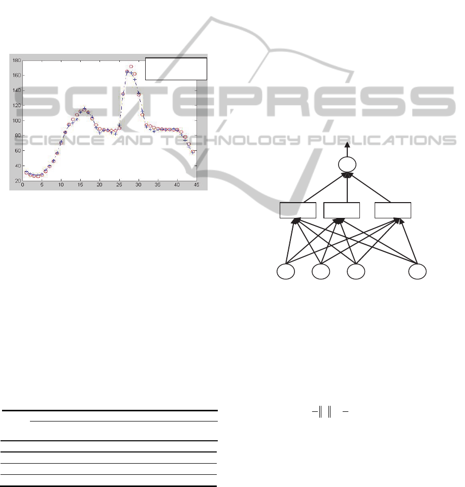
Figure 1: fitting curve of actual values and predict values
of Chl-a in measuring points.
From the results of network training, when sp=10,
network can not converge to expected precision with
bad fitting ability.
If reduce the width of radial basis, network can
converge to goal precision. Its fitting curves with
different widths are shown as follows. In Fig.1, y-
axis is Chl-a (mg/L), x-axis is samples.
There are much difference among generalization
abilities of network and predict results of testing
data with different widths of basis functions. 4
groups of testing data were used to predict in
networks trained with different widths. Results are
as Tab.1.
Table 1.
Testing
data
sp=1 sp=0.6 sp=0.16
Absolute
error
Relative
error
A
b
solute
error
Relative
error
Absolute
error
Relative
error
Group 1 1.47
5.69%
2.85
11%
0.83
3.22%
Group 2 0.69
2.68%
5.18
20.15%
1.13
4.4%
Group 3 7.41
29.68%
3.18
12.74%
0.49
1.97%
Group 4 13.96 59.15 2.61
11.1%
0.24
1%
From Tab.1, it can be seen that: when sp=0.16,
the test error of network is smallest; the approaching
ability and fitting performance are good; network
training is successful.
Network trained can be used to predict the
change of Chl-a at measuring points correctly,
which shows that the network is of strong
generalization and can achieve the expected goal.
Fig.4 shows the curves of actual values and predict
values, where y-axis is Chl-a (mg/L) and x-axis is
sample.
3 MEDIUM-TERM PREDICTING
METHOD BASED ON SUPPORT
VECTOR MACHINE
3.1 Least Squares Support Vector
Machine
Principle of Support Vector Machine (SVM) can be
expressed as following Fig2 (Dominique and
Alistair, 2003).
……
X1 X2 X3 Xn
K ( X1, X )
K ( X2, X )
K ( Xn, X )
A1Y1 A2Y2 AnYn
F(x)
Predict Function
Weigh Value
Core
Calculator
Support Vector
Figure 2: Principle scheme of Support Vector Machine.
As development and improvement of classical
SVM, Least Squares Support Vector Machine
(LSSVM) defines a cost function which is different
from classical SVM and changes its inequation
restriction to equation restriction. In Least Squares
Support Vector Machine, problem of optimization
become as follow (Li Ren et al., 2004):
2
2
,,
1
1
min ( , , )
22
.. ( ) 1,2, , )
l
i
wb
i
T
iii
c
Lwb w
st y w x b i l
(
(10)
Using lagrangian multiplier method to solve the
formulas:
Extreme point of Q is saddle point, and
differentiating Q can obtain formulas as follow:
○Actual Value
●Predict Value
ICAART2013-InternationalConferenceonAgentsandArtificialIntelligence
594
1
1
() 0
0
() 0
0
l
ii
i
l
i
i
T
iii
ii
i
Q
wx
w
Q
b
Q
wxb y
Q
C
(11)
From formulas above:
2
11 111
11
() ()
22
ll lll
ii j j i i ii
ij iii
x
xby
C
(12)
The formula above can be expressed in matrix
form:
1
(1)(1)
0
0
T
ll
b
e
Y
eCI
(13)
In this equation,
1
[1, ,1]
T
l
e
,
(, ) () ( )
T
ij i j i j
Kx x x x
(14)
3.2 Data Pretreatment and Modeling
The outbreak of water bloom usually occurs in
summer, and 100 groups of monitoring data are
selected to established LSSVM water bloom
prediction model
Radial basis functionand, Polynomial core
function, and multi-layer Sigmoid function are
frequently used as core functions. Compared with
the abilities of all kinds of core functions, the ability
of RBF core function is proved to be best among all
core functions
[11]
. Thus core function is as following.
2
2
,
2
k
k
x
x
Kx x
(15)
In the formula,
2
2
1
n
kk
ki
i
x
xxx
(16)
Here
is core width.
LSSVM prediction model based on RBF core
function contains two important parameters:
regularization parameter gam and RBF core function
parameter sig2 Then after combining M·N (gam
,
sig2 ) sets, different LSSVMs are trained
respectively so as to gain a set which has minimum
mean absolute error in those M·N (gam
,
sig2)
sets. This set could be used as optimized parameter.
The result of optimized parameters is as Table 3.
3.3 Establishment of Prediction Model
The structure of LSSVM prediction model is as
follow:6 input variables: temperature T, dissolved
oxygen DO, illumination intensity, total phosphorus
TP, total nitrogen TN and chlorophyll Chl-a. One
output variable is Chl-a;
Parameter optimization function: tunelssvm ( )
3.4 Analysis of Prediction Result
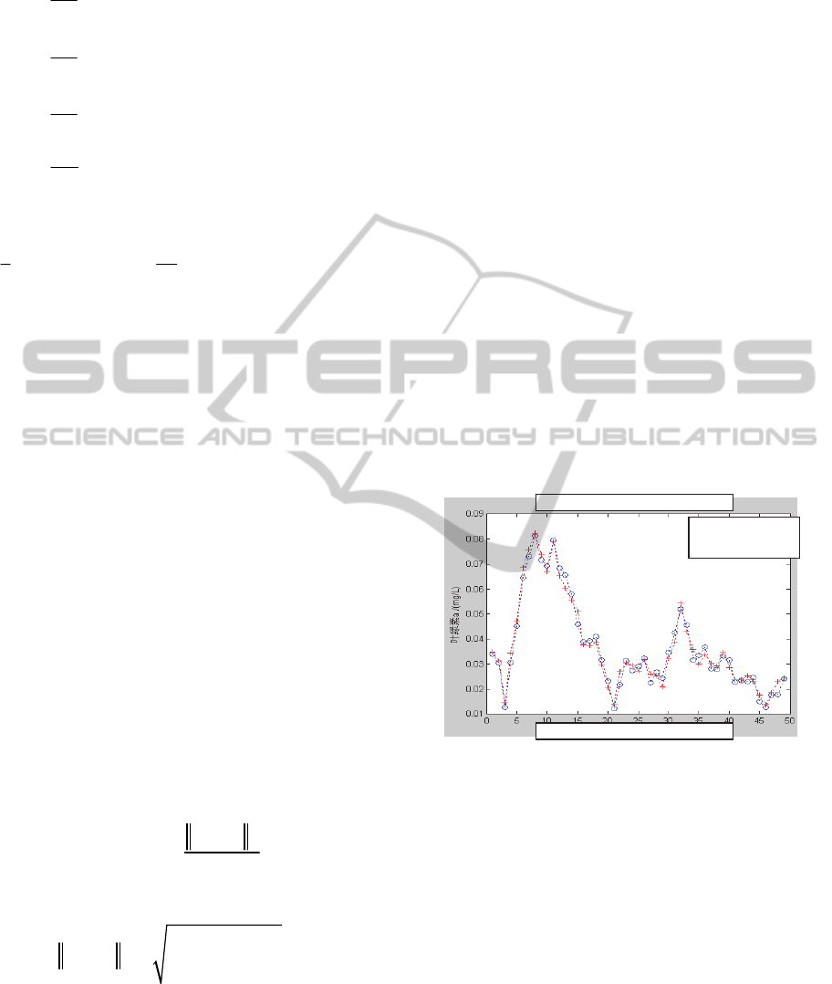
100 groups of water quality monitor data which have
been normalized are substituted in LSSVM water
bloom prediction model of rivers and lakes. Among
them, 50 groups are used for model training, and
other 50 groups are used to predict the content of
Chl-a two days later in model prediction. Prediction
result is as Fig. 3.
Figure 3: Chl-a value two days later in LSSVM prediction
model.
4 PREDICTION RESULTS
COMPARE WITH DIFFERENT
MODEL
On the other hand, classical regression support
vector machine and frequently-used RBF neural
network are respectively used to established water
bloom prediction model. Prediction accuracy of
LSSVM, SVM, RBF are shown in Table 2.
From Table 2, prediction accuracy of LSSVM is
higher than that of SVM whose prediction accuracy
is higher than RBF neural network. LSSVM is
improved based on SVM in algorithm so that its
Real value and
p
rediction value
Prediction value via ever
y
da
y
+ Actual Value
○ Predict Value
IntelligentPredictingMethodofWaterBloombasedRBFNNandLSSVM
595
function generalization ability is greatly enhanced;
RBF neural network is widely used which has good
prediction accuracy in short-term water bloom
prediction. But
as the prediction period increases, its prediction
accuracy will be affected to some extent.
Table 2: Prediction accuracy comparison between LSSVM,
SVM and RBF.
Prediction
accuracy
LSSVM SVM RBF
Chl_a value two
days later after
prediction
94. 23%
82.
64%
72.
58%
From Table 2, prediction accuracy of LSSVM is
higher than that of SVM whose prediction accuracy
is higher than RBF neural network. LSSVM is
improved based on SVM in algorithm so that its
function generalization ability is greatly enhanced;
RBF neural network is widely used which has good
prediction accuracy in short-term water bloom
prediction. But as the prediction period increases, its
prediction accuracy will be affected to some extent.
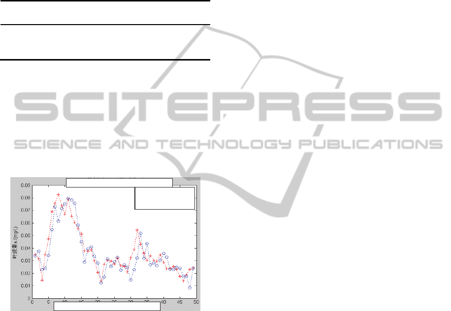
Figure 4: Chl-a value two days later in SVM.
5 CONCLUSIONS
After analyzing and discussing the main factors, two
kinds of short-term and medium-term intelligent
predicting models of water bloom based on RBF
neural networks and LSSVM respectively
researched, and also analyzed and compared with
each other.
First, short- term predict method of water bloom
based on RBF network is put forward, including
research on the monitoring learning algorithms to
the center, width and weight of basis function of
RBF network, as well as error-corrected algorithm
based on gradient descent. The function and
influence, which the number of RBF hidden level
nodes brings to the performance of network, are
analyzed; the width of RBF and fitting and
generalization abilities of network are analyzed and
compared. According to the training and predict
results, the short- term change of Chl-a can be
predicted by using RBF neural network; soft sensing
model of water bloom based on RBF has strong
generalization ability, high predict precision and
good fitting performance, so that an newly effective
method can be provided to predict water flower in
short time.
Then LSSVM is approached, which improves the
algorithm of SVM., and it needs a small amount of
samples, has long-term prediction period, strong
generalization ability and high prediction accuracy.
From the results of models, the fitting precision of
models is relatively good, and it can better predict
the medium-term change rule of Chlorophyll and
provide a new efficient way for water bloom
medium-term intelligent prediction.
ACKNOWLEDGEMENTS
Supported by Beijing Natural Science Foundation
(8101003), National Natural Science Foundation of
China (51179002), and the Beijing Municipal
Commission of Education (PHR201007123,
PHR201008238) and the Beijing Municipal
Commission of Education Science and Technology
Foundation Project.
REFERENCES
Welch E B. Spyridakis D E. Shuster J. Declining lake
sediments phosphorus release and oxygen diversion
Journal of Water Pollution Control Fedration . 1986.
58(1) :92-96.
Somlyody L. Eutrophication modeling, management and
decision making: the Kis-Balaton case. Water Science
and Tecnology, 1998,37(3):165-175.
Vollenweider R A. Input-Output Models with Special
Reference to the Phosphorus Loading Concept in
Limnology. Schweizeische Zeitschrift Hydrol,
1975,37:53—84.
Guisen Du, Yumei Wu, Zhongshan Yang, etc. Analysis of
Water Quality on Urban Rivers and Lakes in Beijing,
Journal of lake sciences, 2005, 17(4):373 - 377.
Qing Liu. Rough set and rough reasoning, Beijing Science
Press. Beijing. 2001, 12-15.
Wu H J, Lin Z Y and Guo S L. Application of artificial
neural network in predicting resources and environment.
Resource and Environment in the Yangtze Basin,
Prediction value via ever
y
da
y
Real value and
p
rediction value
+ Actual Value
○ Predict Value
ICAART2013-InternationalConferenceonAgentsandArtificialIntelligence
596

2000,9(2):237-241.
Van Gestel T, Suykens J, Viacne S, etc. Benchmarking
least squares support vector machine classifiers,
Machine Learning, 2004, 54(1): 5-32.
Zaiwen Liu. Prediction technique for water-bloom in lakes
based on elman network, 2009 IEEE International
Conference on Automation and Logistics, 2009 08
Dominique M, Alistair B. Nonlinear blind source
separation using kernels. IEEE Trans. on Neural
Networks, 2003, 14(1): 228 -235.
Li Ren, Shaohua Li, etc: Application of artificial neural
network model to assessment of Taihu Lake
eutrophication, Journal of Hohai University (Natural
Sciences ), 2004, 32(2):147 – 150.
Suykens J A K,Vandewalle J . Least squares support
vector machine classifiers. Neural Processing Letter,
1999, 9(3):293-300.
IntelligentPredictingMethodofWaterBloombasedRBFNNandLSSVM
597
