
Parametric Macromodeling using Interpolation of Sylvester based
State-space Realizations
Elizabeth Rita Samuel, Luc Knockaert and Tom Dhaene
Department of Information Technology, Ghent University, Gaston Crommenlaan 8 Bus 201, B-9050 Gent, Belgium
Keywords:
Sylvester Equation, Parametric Macromodeling, State-space Matrices, Rational Approximation, Interpolation.
Abstract:
A novel state-space realization for parametric macromodeling is proposed in this paper. A judicious choice
of the state-space realization is required to account for the generally assumed smoothness of the state-space
matrices with respect to the design parameters. This is used in combination with suitable interpolation schemes
to interpolate a set of state-space matrices, and hence the poles and residues indirectly, in order to build
accurate parametric macromodels. The key points are the choice of a proper pivot matrix and the solution
of a Sylvester equation for pole placement. Pertinent numerical examples validate the proposed state-space
realization for parametric macromodeling.
1 INTRODUCTION
When designing a system, or implementing a con-
troller to augment to an existing system the basic step
is to obtain a mathematical model. For this, design
space exploration, design optimization, and sensitiv-
ity analysis are usually performed and this requires
multiple simulations for different design parameter
values (e.g., layout features). Parametric macromod-
eling is an efficient and accurate tool to perform these
design activities, while avoiding new measurements
or simulations for each new parameter configuration.
Parametric macromodels are multivariate models that
describe the complex behavior of the systems, typi-
cally characterized by frequency (or time) and sev-
eral geometrical and physical design parameters, such
as layout or substrate features. Recently, parametric
macromodeling techniques which are able to guaran-
tee overall stability and passivity have been proposed
in (Ferranti et al., 2010a; Deschrijver and Dhaene,
2008; Ferranti et al., 2009; Ferranti et al., 2010b;
Triverio et al., 2010) . The techniques described in
(Ferranti et al., 2010a) and (Ferranti et al., 2009)
are based on the interpolation of a set of univariate
macromodels, called root macromodels. This inter-
polation process of input-output systems leads to pa-
rameterization of the residues, but unfortunately not
of the poles. Passive interpolation of the state-space
matrices of a set of root macromodels is proposed
in (Ferranti et al., 2010b) and(Triverio et al., 2010),
providing an increased modeling capability with re-
spect to (Ferranti et al., 2010a) and (Ferranti et al.,
2009), due to the parameterization of both poles and
residues. Unfortunately, these methods are sensitive
to issues related to the interpolation of state-space ma-
trices (De Caigny et al., 2009), such as the smooth-
ness of the state-space matrices as a function of the
parameters.
In this paper, we propose a novel state-space re-
alization that is suitable to build accurate parametric
macromodels. The direct parameterization of poles
and residues is avoided, due to their potentially non-
smooth effect with respect to the design parameters.
A conversion from a pole-residue form obtained by
means of Vector Fitting (VF) (Gustavsen and Sem-
lyen, 1999) to a Sylvester realization is computed for
each root macromodel. Since the same pivot (refer-
ence) matrix is used for all state-space realizations of
the root macromodels, smooth variations of the state-
space matrices with respect to the design parameters
are expected. It leads to build accurate parametric
macromodels using suitable interpolation schemes.
We focus on applications described by scattering
(S) parameters, but the approach can be also used
for other system representations, e.g. admittance and
impedance parameters. Pertinent numerical exam-
ples validate the proposed state-space realization for
macromodeling.
319
Rita Samuel E., Knockaert L. and Dhaene T..
Parametric Macromodeling using Interpolation of Sylvester based State-space Realizations.
DOI: 10.5220/0004401603190325
In Proceedings of the 10th International Conference on Informatics in Control, Automation and Robotics (ICINCO-2013), pages 319-325
ISBN: 978-989-8565-70-9
Copyright
c
2013 SCITEPRESS (Science and Technology Publications, Lda.)

2 PARAMETRIC
MACROMODELING
Starting from a set of M data samples
{(s,~p)
k
,H(s,~p)
k
}
M
k=1
, a set of frequency-dependent
rational models is built for some design space
points by means of system identification techniques
(Pintelon et al., 1994), in our case the VF technique
(Gustavsen and Semlyen, 1999). The result of
this initial procedure is a set of rational univariate
macromodels with Gilbert realization, called root
macromodels. Each root macromodel is related to
a root point ~p = (p
(1)
k
1
,..., p
(M)
k
M
) in the design space.
Two data grids are used in the modeling process:
an estimation grid and a validation grid. The first
one is utilized to build the root macromodel which,
combined with an interpolation scheme, provide
the parametric macromodel. The second grid, more
dense than the previous one, is utilized to assess the
interpolation capability of the parametric macro-
model, its capability of describing the system under
study in points of the design space previously not
used for the construction of the root macromodel.
Suppose we have a set of models S
~p
k
, k =
1,....,N with given minimal realizations
S
~p
k
≡
A
~p
k
B
~p
k
C
~p
k
D
~p
k
, (1)
state-space equations
˙x = A
~p
k
x + B
~p
k
u (2)
y = C
~p
k
x + D
~p
k
u (3)
and transfer functions
R
~p
k
(s) = C
~p
k
(sI − A
~p
k
)
−1
B
~p
k
+ D
~p
k
(4)
In this paper we suppose that all realizations S
~p
k
have
the same McMillan degree N and number of ports
P ≤ N. We further suppose that all matrices A
~p
k
are
Hurwitz stable.
We propose a generic parametric realization of the
form
S (~p) ≡
A(~p) B(~p)
C(~p) D(~p)
(5)
with ~p = (~p
(1)
,...,~p
(M)
). The models S
~p
k
can be con-
sidered as snapshots of S (~p) generated by fixing the
parameter ~p at the fixed values ~p
k
. S
~p
k
must be able
to accurately model the system behavior as a function
of s and ~p.
3 STATE-SPACE REALIZATION
To obtain accurate parametric macromodels by inter-
polating the state-space matrices, the realization is
very important.
In what follows, we discuss the well-known
Gilbert and Balanced realizations, and the proposed
novel Sylvester realization.
3.1 Gilbert Realization
The minimal state-space realization problem for lin-
ear time invariant (LTI) systems was first stated by
Gilbert (Gilbert, 1963), who gave an algorithm for
transforming a transfer function into a system of dif-
ferential equations (i.e. a state-space description).
The approach of Gilbert is based on partial-fraction
expansions. In the Gilbert approach the poles and the
residues are stamped directly in the state-space matri-
ces and since poles and residues may present a highly
non-smooth behavior with respect to design parame-
ters, achieving a high accuracy in parametric macro-
models built by interpolation of state-space matrices
becomes difficult.
3.2 Balanced Realization
A minimal and stable realization is called balanced
(Moore, 1981; Pernebo and Silverman, 1982) if
the controllability and observability Gramians are
equal and diagonal. Every minimal system can be
brought into balanced form. The balanced realiza-
tion can be implemented using the Matlab function
balreal. This routine uses the eigen decomposition
of the product of the observability and controllability
Gramians to construct the balancing transformation
matrix. As stated in (De Caigny et al., 2009; Peeters
et al., 2009), uniqueness is guaranteed up to a sign
and it may effect the smoothness of the state-space
matrices as functions of design parameters.
The problem with the interpolation procedure
for the Gilbert and balanced realization is that, al-
though the interpolation technique yields (by con-
struction) the discrete macro-model S
~p
k
for ~p = ~p
k
,
it is not at all sure that the interpolated matrices
A(~p),B(~p),C(~p),D(~p) will behave smoothly between
the nodes p
k
. The reason for this is that minimal real-
izations are all equivalent modulo a similarity trans-
formation, i.e., two realizations related by
˜
A
~p
k
˜
B
~p
k
˜
C
~p
k
˜
D
~p
k
=
X
−1
A
~p
k
X X
−1
B
~p
k
C
~p
k
X D
~p
k
(6)
where X is any nonsingular matrix, yield the same
transfer function
H(s) = C
~p
k
(sI − A
~p
k
)
−1
B
~p
k
+ D
~p
k
=
˜
C
~p
k
(sI −
˜
A
~p
k
)
−1
˜
B
~p
k
+
˜
D
~p
k
(7)
It is important to note that the interpolation of
state-space matrices allows a higher modeling capa-
ICINCO2013-10thInternationalConferenceonInformaticsinControl,AutomationandRobotics
320

bility than the interpolation of transfer functions (Fer-
ranti et al., 2010a; Ferranti et al., 2009), but unfortu-
nately these methods are sensitive to issues related to
the smoothness of the state-space matrices as a func-
tion of the parameters. In the following subsection,
the novel realization can guarantee smoothness since
they are pivot-based realizations.
3.3 Sylvester Realization
We propose the following state-space feedback real-
ization with feedback matrix F and pivot matrix
˜
A
˙x =
˜
Ax +
˜
B
~p
k
v (8a)
y =
˜
C
~p
k
x +
˜
D
~p
k
v (8b)
v = −Fx + u (8c)
where
˜
A is a fixed N × N pivot matrix and F is a fixed
p × N state-space feedback matrix. This realization
can be written as
R
~p
k
≡
˜
A −
˜
B
~p
k
F
˜
B
~p
k
˜
C
~p
k
−
˜
D
~p
k
F
˜
D
~p
k
(9)
For R
~p
k
and S
~p
k
to be equivalent, the existence of non-
singular matrices X
k
such that
˜
A −
˜
B
~p
k
F = X
−1
k
A
~p
k
X
k
(10a)
˜
B
~p
k
= X
−1
k
B
~p
k
(10b)
˜
C
~p
k
= C
~p
k
X
k
(10c)
is needed.
By eliminating (10b) from (10a) we obtain the
Sylvester equation
A
~p
k
X
k
− X
k
˜
A + B
~p
k
F = 0 (11)
for the unknown matrix X
k
. We need the following
Theorem 1. The Sylvester equation (11) has a unique
nonsingular solution X
k
provided the pair (A
~p
k
,B
~p
k
)
is controllable, the pair (
˜
A,F) is observable, and the
intersection of the eigenspectra of A
~p
k
and
˜
A is empty.
Proof. See (de Souza and Bhattacharyya, 1981;
Varga, 2000).
Note that Sylvester equations are routinely solved
by the Matlab function lyap.
Remark 1. The Sylvester realizations given the pivot
matrix
˜
A and feedback matrix F, are all unique by
construction. For the choice of
˜
A we can take a block-
diagonal or block-Jordan matrix(Varga, 2000) which
never shares eigenvalues with any of the A
~p
k
matrices.
This can be accomplished by choosing the eigenval-
ues of
˜
A close to the imaginary axis (see also the nu-
merical simulations). The choice of F is subject to the
requirement that the pair (
˜
A,F) has to be observable.
In some cases such as the Gilbert (Gilbert, 1963) or
Vector Fitting (Gustavsen and Semlyen, 1999) real-
ization, all matrices B
k
are equal, and then a judi-
cious choice for F is F = B
T
k
. In the Appendix we
show that, under very general conditions, there ex-
ist realizations such that all B
k
are equal. More gen-
erally speaking, F can be chosen quite freely, or its
choice can be imbedded in the overall Sylvester algo-
rithm (Carvalho et al., 2003).
4 NUMERICAL EXAMPLES
In the following examples, we show the importance
of the realization issue, and validate the proposed
Sylvester approach, by comparing them with the stan-
dard Gilbert and balanced realizations.
4.1 Two Coupled Microstrip with
Variable Length (CM)
Two coupled microstrips can be modeled (Knockaert
and De Zutter, 2000) starting from per-unit-length pa-
rameters. The cross section is shown in Figure.1.
Figure 1: CM: Two coupled microstrip line.
Figure 1 shows its cross section. The length L are
considered as variable parameters in addition to fre-
quency. Their corresponding ranges are shown in Ta-
ble 1.
Table 1: CM: Parameters Of The Coupled Microstrips.
Parameter Min Max
Frequency ( f req) 20 MHz 8 GHz
Length (L) 2.5 cm 3 cm
The scattering parameters were obtained over a
validation grid of 200×11 samples, for frequency and
length respectively. We have built root macromodels
for 6 values of the spacing by means of VF, each with
an order 11.
As described in Section 3.3, a pivot matrix
and a feedback matrix is chosen such that a well-
conditioned solution is obtained for the Sylvester
ParametricMacromodelingusingInterpolationofSylvesterbasedState-spaceRealizations
321
equation (11). We use a VF form of pivot matrix
(Gustavsen, ), which can be coded in Matlab as
N ; % Order of approximation
%Complex conjugate pairs, linearly
spaced:
bet=linspace(w(1),w(end),N/2);
poles=[];
for n=1:length(bet)
alpha=-beta(n)*1e-2;
poles=[poles (alpha-i*beta(n))
(alpha+i*beta(n)) ];
end
i.e; the pole pairs are chosen as
a
n
= −α + jβ, a
n
= −α − jβ
where, α = β/100.
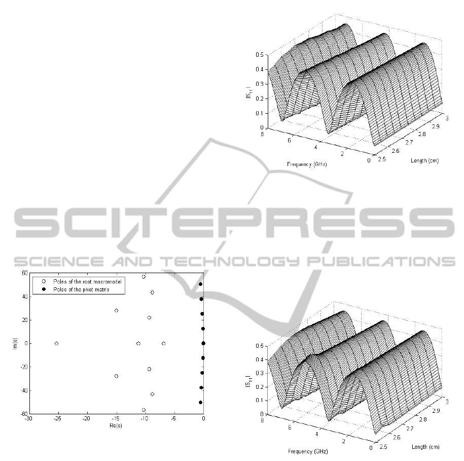
Also, since the eigenvalues of the pivot matrix and
those of the root macromodels obtained from Gilbert
realization must not be the same, we choose the poles
very close to the imaginary axis as shown in Figure 2.
Figure 2: CM: Eigenvalues of the pivot matrix and the root
macromodels obtained from Gilbert realization.
The feedback matrix is chosen as column vec-
tors of 1’s, 2’s and 0’s similar to VF technique. A
similarity transformation is then performed using the
Sylvester solution to obtain the state-space matrices
of the Sylvester realization.
Finally, a bivariate macromodel is obtained by
linear interpolation of the corresponding state-space
matrices using the Sylvester realization as shown in
Figure.3.
The maximum absolute error over the validation
grid for the parametric macromodel of the scattering
matrix is bounded by −56 dB. It can be noted that
a very good agreement is obtained between the origi-
nal data and the proposed parametric macromodeling
technique. The parametric macromodel captures the
Figure 3: CM: Magnitude of the bivariate macromodel
S
11
(s,L) (Sylvester realization for each root macromodel).
behavior of the system very accurately over the entire
range of the length.
Figure.4 shows that direct parameterization of
the poles should be avoided due to potentially non-
smooth behavior with respect to the design parame-
ters with Gilbert realization.
Figure 4: CM: Magnitude of the bivariate macromodel
S
11
(s,L) (Gilbert realization form for each root macro-
model).
In Figure 5 it is shown that the maximum absolute
error is very small for the Sylvester but it is not satis-
factory for the Gilbert and balanced real realization.
4.2 Hairpin Bandpass Microwave Filter
(HP)
In this example, a hairpin bandpass filter with the lay-
out shown in Figure.6 is modeled. The relative per-
mittivity of the substrate is 9.9, and its thickness is
equal to 0.635 mm.
ICINCO2013-10thInternationalConferenceonInformaticsinControl,AutomationandRobotics
322
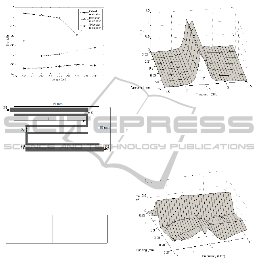
Figure 5: CM: Absolute error comparison for the different
realizations.
Figure 6: HP: Layout of the Hairpin bandpass microwave
filter.
The spacing S
1
and the length L of the stub are chosen
as design variables in addition to frequency. Their
corresponding ranges are shown in Table 2.
Table 2: HP: Parameters Of The Hairpin Bandpass Mi-
crowave Filter.
Parameter Min Max
Frequency ( f req) 1.5 GHz 3.5 GHz
Length (L) 12 mm 12.5 mm
Spacing (S
1
) 0.27 mm 0.32 mm
The scattering parameters have been computed by
means of the advanced design system (ADS) over a
grid of 11 × 7 samples, for length and spacing respec-
tively. We have built root macromodels for 6 × 4 val-
ues of the length and spacing respectively by means
of VF, each with an order 13. Next the realization
approaches as described in Section 3.3 is used to ob-
tain Sylvester realized state-space form for each root
macromodel. Finally, a trivariate macromodel is ob-
tained by multilinear interpolation of the correspond-
ing state-space matrices as shown in Figure 7.
The maximum absolute error over the validation
grid for the parametric macromodel of the scattering
matrix is bounded by −58 dB. It can be noted that
a very good agreement is obtained between the origi-
nal data and the proposed parametric macromodeling
technique. The parametric macromodel captures the
Figure 7: HP: Magnitude of the trivariate macromodel
S
12
(s,L,S) for L = 12.05 mm (Sylvester realization for each
root macromodel).
behavior of the system very accurately over the entire
design space.
Figure 8 shows the parametric macromodel using
balanced real realization. It is seen by comparing with
Figure 7 that the behavior is very erratic.
Figure 8: HP: Magnitude of the trivariate macromodel
S
12
(s,L,S) for L = 12.05 mm (Balanced realization for each
root macromodel).
For the hairpin filter it can be also noted from the Fig-
ure 9 that the maximum absolute error is very small
for the Sylvester realization but it is not satisfactory
for Gilbert realization and balanced real realization.
5 CONCLUSIONS
This paper proposes a novel state-space realization
for parametric macromodeling. For the generally as-
sumed smoothness of the state-space matrices with
ParametricMacromodelingusingInterpolationofSylvesterbasedState-spaceRealizations
323

Figure 9: HP: Absolute error comparison for the different
realizations.
respect to the parameters a wise choice of the state
space realization is required. This realization is used
in combination with suitable interpolation schemes
to interpolate the set of state-space matrices in order
to build accurate parametric macromodels. The key
point is to find a suitable pivot matrix and to solve
Sylvester equations such that well conditioned solu-
tion are obtained. From the numerical examples it is
seen that the proposed realization technique generates
a more accurate parametric model with respect to the
design parameters in comparison to the Gilbert real-
ization and balanced realization.
ACKNOWLEDGEMENTS
This work was supported by the Research Foundation
Flanders (FWO) and by the Interuniversity Attraction
Poles Programme BESTCOM initiated by the Belgian
Science Policy Office.
REFERENCES
Carvalho, J., Datta, K., and Hong, Y. (2003). A new
block algorithm for full-rank solution of the sylvester-
observer equation. IEEE Transactions on Automatic
Control, 48(12):2223 – 2228.
De Caigny, J., Camino, J. F., and Swevers, J. (2009). Inter-
polating model identi- cation for siso linear parameter-
varying systems. Mechanical Systems and Signal Pro-
cessing, 23(8):2395–2417.
de Souza, E. and Bhattacharyya, S. (1981). Controllability,
observability and the solution of AX -XB = C. Linear
Algebra and its Applications, 39:167 – 188.
Deschrijver, D. and Dhaene, T. (2008). Stability and passiv-
ity enforcement of parametric macromodels in time
and frequency domain. IEEE Transactions on Mi-
crowave Theory and Techniques, 56(11):2435 –2441.
Ferranti, F., Knockaert, L., and Dhaene, T. (2009). Parame-
terized S-parameter based macromodeling with guar-
anteed passivity. IEEE Microwave and Wireless Com-
ponent Letters, 19(10):608–610.
Ferranti, F., Knockaert, L., and Dhaene, T. (2010a). Guaran-
teed passive parameterized admittance-based macro-
modeling. IEEE Transactions on Advanced Packag-
ing, 33(3):623 –629.
Ferranti, F., Knockaert, L., Dhaene, T., and Antonini, G.
(2010b). Passivity-preserving parametric macromod-
eling for highly dynamic tabulated data based on
Lur’e equations. IEEE Transactions on Microwave
Theory and Techniques, 58(12):3688 –3696.
Gilbert, E. G. (1963). Controllability and observability in
multi-variable control systems. SIAM Journal on Con-
trol, 1(2):128–151.
Gustavsen, B. USERS GUIDE FOR vectfit3.m (Fast, Re-
laxed Vector Fitting) for Matlab.
Gustavsen, B. and Semlyen, A. (1999). Rational approxi-
mation of frequency domain responses by vector fit-
ting. IEEE Transaction on Power Delivery, 14:1052–
1061.
Knockaert, L. and De Zutter, D. (2000). Laguerre-SVD
reduced-order modeling. IEEE Transactions on Mi-
crowave Theory and Techniques, 48(9):1469 –1475.
Moore, B. (1981). Principal component analysis in lin-
ear systems: Controllability, observability, and model
reduction. IEEE Transactions Automatic Control,
26(1):17–31.
Peeters, R., Olivi, M., and Hanzon, B. (2009). Balanced
realization of lossless systems: Schur parameters,
canonical forms and applications. 15th IFAC Sympo-
sium on System Identification, pages 273–283.
Pernebo, L. and Silverman, L. M. (1982). Model reduction
via balanced state space representations. IEEE Trans-
actions Automatic Control, 27(2):382–387.
Pintelon, R., Guillaume, P., and Rolain, Y. (1994). Paramet-
ric identification of transfer functions in the frequency
domain- A survey. IEEE Transactions on Automatic
Control, 39(11):2245–2260.
Triverio, P., Nakhla, M., and Grivet-Talocia, S. (2010). Pas-
sive parametric modeling of interconnects and pack-
aging components from sampled impedance, admit-
tance or scattering data. Electronic System-Integration
Technology Conference, pages 1–6.
Varga, A. (2000). Robust pole assignment via sylvester
equation based state feedback parametrization. Pro-
ceedings of the IEEE International Symposium on
Computer-Aided Control System Design, pages 13–
18.
ICINCO2013-10thInternationalConferenceonInformaticsinControl,AutomationandRobotics
324

APPENDIX
We need to prove that, given a matrix
˜
B, there exists
a nonsingular matrix T
k
such that T
−1
k
B
k
=
˜
B. The re-
sulting equivalent realization is then
T
−1
k
A
k
T
k
˜
B
C
k
T
k
D
k
(12)
This is proved under quite general circumstances by
the following theorem :
Theorem 2. Let n ≥ m and B,
˜
B n × m full rank ma-
trices. Then the matrix equation T
˜
B = B admits a
nonsingular n × n matrix solution T.
Proof. First suppose n = m. Then T = B
˜
B
−1
is non-
singular. Next suppose m < n. Consider the QR de-
compositions of B and
˜
B :
B = Q
R
0
˜
B = Q
1
R
1
0
(13)
Then the matrix
T = Q
RR
−1
1
0
0 Y
Q
T
1
(14)
with Y nonsingular, is itself nonsingular, and satisfies
T
˜
B = Q
R
0
= B (15)
The proof is complete. Note that for simplicity we
can take Y = I
n−m
.
ParametricMacromodelingusingInterpolationofSylvesterbasedState-spaceRealizations
325
