
The Parameter Optimization in Multiple Layered Deduplication System
Mikito Ogata
1
and Norihisa Komoda
2
1
Hitachi Computer Peripherals Co., Ltd., 781 Sakai, Nakai-machi, Ashigarakami-gun, 259-0180, Kanagawa, Japan
2
Osaka University, 2-1 Yamadaoka, Suita, 565-0824, Osaka, Japan
Keywords:
Deduplication, Backup, Capacity Optimization, Enterprise Storage.
Abstract:
This paper proposes a multiple layered deduplication system for backup operation in IT environment. The
proposed system reduces the duplication in data by using a series of algorithms which are installed with
different chunk sizes in descendent order. Our research defines the models and formula for the cumulative
deduplication rate and processing time over multiple layers of the system, then, points out the efficiency is
heavily affected by how to assign the chunk sizes in each layer in order to achieve the optimal assignment.
Finally, the efficiency of the proposal is compared to a conventional single layer deduplication system to assure
the improvement.
1 INTRODUCTION
Due to the explosive increase of the data in IT sys-
tem, the resource usage, the processing time and the
managing cost for backup operation are becoming a
burden to the system, while it is recognized as an in-
dispensable operation to protect the data in case of
unpredictable disaster. Major requirements to backup
operations are to shorten the processing time and to
reduce the resource usage, especially storage capac-
ity. Recently, the technology called deduplication has
become popular to reduce the burden. This is a tech-
nology to eliminate the duplication of the backup tar-
get data and store only unique data in the storage. The
reduction of stored data reduces not only the backup
storage cost but also other resources running work-
load. Various techniques have been proposed so far
to provide more deduction with less processing time
from the point view of more cost-effective backup op-
eration(Y. Tan et al., 2010)(Y. Won et al., 2008)(B.
Zhu et al., 2008). However, the trade-off between the
improvement of the rate and the time makes it diffi-
cult to improve both rate and time simultaneously.
This paper points out the trade-off is hard to over-
come only by using single layer deduplication sys-
tem, then, proposes the multiple layered deduplica-
tion system breaks the trade-off and achieves higher
efficiency than the conventional one. We make the
formula to represent the efficiency, then, define Pareto
optimal solution and analyze the tendency of the af-
fection of chunk sizes of each layer in order to max-
imize the rate or minimize the processing time, fi-
nally, show the improvement of our proposed method
in comparison to the conventional method.
2 CONVENTIONAL APPROACH
AND THE ISSUES
2.1 Single Layer Deduplication System
The conventional deduplication backup system con-
sists of single module, which has the associated dedu-
plication algorithm. The module analyzes the tar-
get data, identify the segments, distinguish the du-
plicated area from the unique or newly updated area,
then transfer and store only the unique data in the
storage. Backup target data includes various types of
files, such as imaging, documents, compressed files,
structured M2M data and so on. The duplication
level included in the data also depends on the environ-
ments, for example some are scarcely duplicated be-
cause it was much edited, changed or updated, some
are densely duplicated because it was rarely changed,
just replicated or copied, and so on.
Figure 1 shows the typical operational flow of the
deduplicationprocess from reading the targetdata and
finalizing to store the unique data.
The size of the box is not to scale. A
module divides the target data in small segments
called ’Chunk’s which are the unit of reduce or
143
Ogata M. and Komoda N..
The Parameter Optimization in Multiple Layered Deduplication System.
DOI: 10.5220/0004423601430150
In Proceedings of the 15th International Conference on Enterprise Information Systems (ICEIS-2013), pages 143-150
ISBN: 978-989-8565-60-0
Copyright
c
2013 SCITEPRESS (Science and Technology Publications, Lda.)
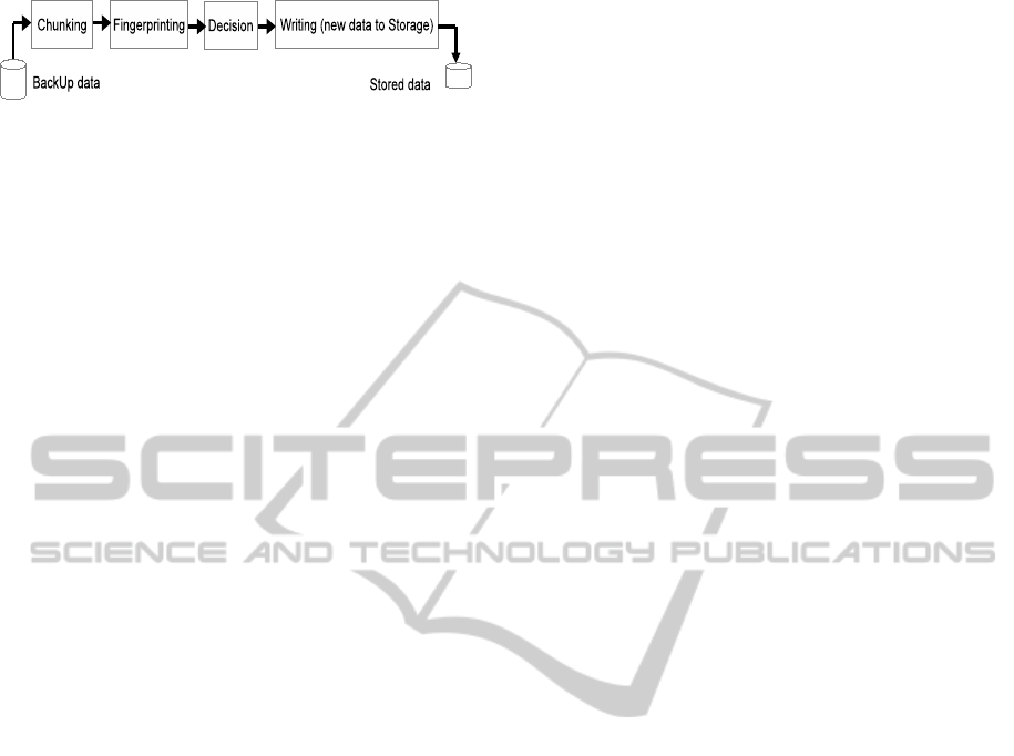
Figure 1: Deduplication process.
store(Chunking). Commonly used dividing mech-
anism is fixed length chunking or variable length
chunking. Fixed length chunking divides the data into
the same length chunks. Variable length chunking
divides into different length chunks. Typical imple-
mentation of variable length chunking scans the data
from the starting bytes to the end in sequence with
short length window using like Rabin’s algorithm(M.
O. Rabin, 1981), then a special value in the window
is recognized as a boundary of the chunks(U. Man-
ber, 1994)(A. Muthitacharoen et al., 2001). This pa-
per call the value ’anchor’. The average chunk size is
defined from how many bits is taken in the window
bandwidth. Next, the module calculates the unique
code from the chunk data to analyze the similarity
of chunks(Fingerprinting). The codes are calculated
for example by SHA-1, SHA-256, MD5 algorithms(J.
Burrows and D. O. C. W. DC, 1995)(R. Rivest, 1992).
This paper call the codes ’fingerprint’. Next the mod-
ule decides the uniqueness of each chunk using the
codes(Decision), such that the chunk is duplicated
that the same chunk has been stored or not duplicated
that all previous chunks are different. Finally, the
module write out only the unique data into the stor-
age(Writing).
Backup target data includes various types of files,
such as images, documents, compressed files, struc-
tured M2M data and so on(N. Park and D J. Lilj,
2010). The duplication level included in the data
also depends on the environments, for example some
are scarcely duplicated because it was much edited,
changed or updated, some are densely duplicated be-
cause it was rarely changed, just replicated or copied,
and so on.
2.2 Issues
Many approaches have been proposed and imple-
mented with the aim of increasing the deduplica-
tion rate and decreasing the processing time. These
approaches are applied only for the improvement
of single layer deduplication system. Some typical
techniques are to choose fixed or variable chunking
method, use bloom filter, construct the layered index
table and become aware of the data contents and so
on(Y. Tan et al., 2010)(C. Liu et al., 2008)(Y. Won
et al., 2008)(B. Zhu et al., 2008). How to choose the
adequate chunk size in practice is a sensitive factor
of the algorithm, because that affects the total sys-
tem behavior. In many cases, it is determined based
on the reasonable balance of the performance and the
deduplication capability for a hypothetical environ-
ment(D. Meister and A. Brinkmann, 2009)(C. Dub-
nicki et al., 2009)(Quantum Corporation, 2009)(EMC
Corporation, 2010)(G. Wallace et al., 2012).
The trade-off between the chunk size and the pro-
cessing time is not easy to overcome. A smaller
chunk size provides more precise reduction of dupli-
cation, a bigger one provides more coarse. At the
same time, a smaller chunk size requires more CPU
and IO intensive processing time, a bigger one does
less time. Further, it is a non-linear correlation, that
is, for a smaller chunk size, the processing time in-
creases more steeply as the size decreases.
On the other hand, in typical user environment,
the time tolerance for backup operation is pre-defined.
The time tolerance is decided to minimize the impact
by an operation for system continuity. One important
factor is a period of time during which backup are
permitted to run. It should be decided to assure the
least interference with normal operations. We call it
as Backup-window. In these cases, even if the system
desires more precise deduplication for reducing the
storing capacity and cost, the Backup-window cannot
allow to use the adequate small size. In practical en-
vironment, bigger chunk size is adapted to maintain
required performance as a compromise.
In addition, smaller chunk size causes disadvan-
tages as well as advantages, for example, the smaller
chunk works efficiently to reduce the duplication in
case that the duplicate area is adequately spread out
across the data, but works inefficiently when the du-
plicate area is heavily or sparsely localized. When the
duplication is heavy or sparse, smaller chunk wastes
the time of chunking and decision. The continuous
appearance of duplicate area or unique area cause less
productive chunking process. In this case, smaller
chunk size is not beneficial in comparison with bigger
chunk size. In typical user environment, periodical
full backup scenario is popular to help a safe disas-
ter recovery, in this situation, the target data includes
a lot of duplicate area, therefore smaller chunk size
may be inefficient. On the other hand, in the situation
when periodical differential backup scenario is used
to reduce a excessive cost, the target data includes du-
plicate area with less density, ex. a half. Thus, the ef-
ficiency of the chunk size depends on the amount and
locality of duplication embedded in the target data.
This makes it difficult to choose the size uniformly
over all different environments.
ICEIS2013-15thInternationalConferenceonEnterpriseInformationSystems
144
3 MULTIPLE LAYERED
DEDUPLICATION SYSTEM
3.1 Overview
Analysis described above indicates it would be bene-
ficial to the system if a new approach can increase the
deduplication rate with less penalty for the processing
time. In addition, if the implementation provides sta-
bility even in case of densely or sparsely duplicated
data, it is useful to configure universal backup sys-
tems over various environments. We propose a multi-
ple layered deduplication system that can reduce the
duplication by using bigger chunk size in case that the
duplication is heavier and by using smaller chunk size
in case that the duplication is lighter.
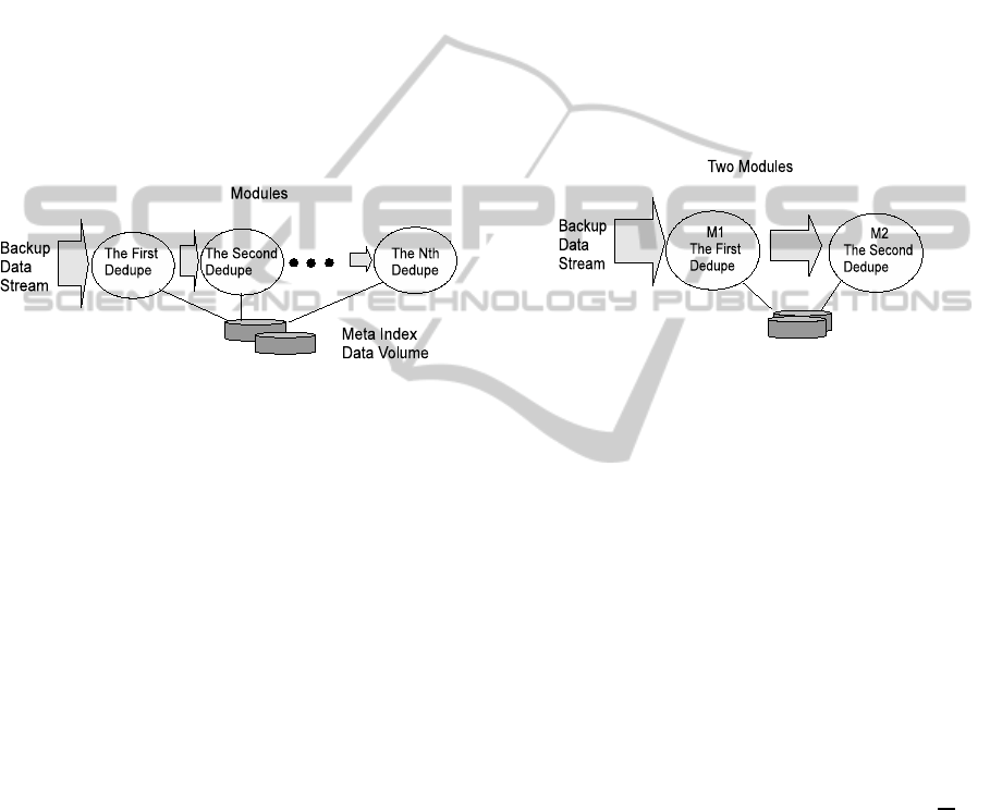
Figure 2: Multiple layered deduplication.
Figure 2 shows the system configuration of multi-
ple layered deduplication system. Backup target data
are deduplicated by a series of modules. Each module
has an independent deduplication algorithm installed.
The data are ingested into the first module for the first
reduction, then the residual data are ingested from the
first module into the second module for the second re-
duction, and the same shall apply hereafter.
Backup target data includes duplicated area,
which is equal to previously stored data, as well as
unique area, which does not match any previous one.
Here, the rate of amount of duplicated area to all of
data is called ’Duplication Rate’. How much data can
be reduced by a module depends on the algorithm in-
stalled in it, especially the chunk size. We implement
the chunk size in descending order over the layers.
The time tolerance is predefined as Backup-window.
In practice, the implementation of multiple lay-
ered deduplication system happen to produce an ex-
cessive capacity tentatively during the process. The
story is that an original data is ingested, duplicated
portion are checked and removed while retaining new
chunks by the first module, then the new chunks are
ingested into the second module. It divides the chunk
in smaller chunks and checks the duplication more
precisely. At first changing timing, which is, the first
time when a chunk is re-chunked by the second mod-
ule after the time when the chunk is stored by the first
module, this may cause an excessive capacity due to
duplicate storing. However spacial locality character-
istic which is inherent in the data eliminate the excess
and recover the inefficiency through the consecutive
generated backup operations.
3.2 Process of Dual Layered
Deduplication System
Theoretically, our proposed system can be configured
with two layers, ex. three layers, four layers, and so
on, howeverfrom the implementation point view, dual
layered configuration which consists of two layers is
practical. Hereafter, we focus on two layers configu-
ration, as a ’dual layered deduplication system’.
Figure 3: Dual layered deduplication.
Figure 3 shows the configuration of dual layered
deduplication system.
M
1
is the first module and M
2
is the second. Both
use variable length chunking method. The target data
is ingested into M
1
first and reduced, then the residual
data after the M
1
reduction is ingested into M
2
and re-
duced. Only the residual data after M
2
are stored in
the final storage as a deduplicated data.
Assuming M
1
has 32KB chunk size with 1ms of
processing time, M
2
has 8KB with 1.25ms. Fig-
ure 4 shows an example of the improvement. The
backup target data is 160KB length, is divided into
five chunks by M
1
variable size chunking and twenty
chunks by M
2
in average. Because the length of each
chunk generally differs due to the chunk boundaries
cut by anchor value, only the average length are as-
sumed. Target data has Duplication Rate of 0.9 (=
18
20
).
Three allocation of modules for target data, such
as M
1
-only, M
2
-only, M
1,2
-combined, provide differ-
ent deduplication rate and processing time, which are
listed in Table 1.
The allocation of M
1,2
-combined provides the
maximum deduplication rate with shorter processing
time than M
2
-only. M
1
-only provides the shortest pro-
cessing time but with less deduplication rate. M
2
-only
has the maximum deduplication rate with the longest
processing time.
As a note for this example, the boundaries of
chunking by M
1
and M
2
do not always match when
TheParameterOptimizationinMultipleLayeredDeduplicationSystem
145
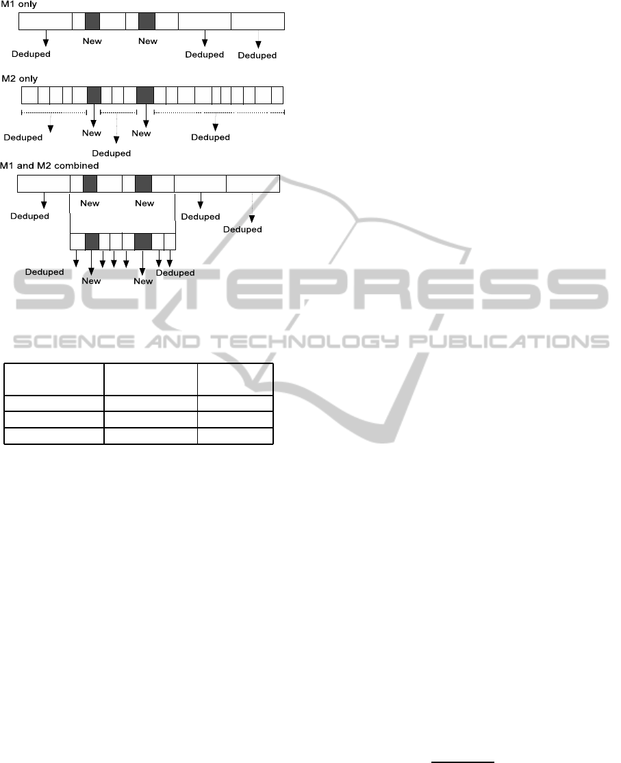
Figure 4: Example of deduplication by two layered method.
Table 1: Total processing time and deduplication ratio by
three allocation scenarios.
Allocation Deduplication Processing
scenario rate [%] time [ms.]
M
1
-only 60 5
M
2
-only 90 25
M
1,2
-combined 90 15
the system use anchor type variable chunkingmethod,
because it cannot assure the identical boundaries for
both.
In above system, the efficiency strongly depends
on the chunk sizes installed in M
1
, M
2
and Duplica-
tion Rate. If M
1
chunk size becomes bigger, M
1
pro-
cessing time is shortened but the deduplication rate
is also decreased. In addition, bigger chunk size in
M
1
causes heavier process in M
2
as a next layer. In
this case, bigger chunk size in M
1
may spoil the ben-
efit of load distribution between the two layers. Con-
versely, if M
1
chunk size become smaller, M
1
pro-
cessing time is increased and the deduplication rate is
also increased. In this case, smaller chunk size in M
1
may spoil the benefit of fast reduction in early layer.
There is the balanced combination of chunk sizes in-
stalled in both M
1
and M
2
. We propose how these
chunk sizes should be chosen to tune the efficiency,
considering the deduplication rate or the processing
time.
4 MODELING OF DUAL
LAYERED DEDUPLICATION
SYSTEM
4.1 System Deduplication Rate (SDR)
and System Processing Time Ratio
(SPT)
The system has two modules as M
i
(i=1,2). Modules
implement SHA type functions for FingerPrinting, a
bloom filter as an initial decision and index tables ma-
nipulating with binary search algorithm. Let D
i
(r) be
a rate of the amount of data that M
i
reduces in the
total amount, called Module Deduplication Rate, and
T
i
(r) be the processing time ratio that M
i
takes, called
Module Processing Time Ratio. For convenience, we
use here a ratio instead of an absolute time value for a
module processing time without losing generality, be-
cause the time varies depending on the data amount or
the system configuration. The base of the ratio can be
chosen in many ways, here we use the value of a to-
tal processing time except a decision time, because all
processes other than decision are considered indepen-
dent from the chunk size and therefore takes relatively
constant time. On the other hand, the decision time is
heavily depends on the chunk size. We assign the ex-
act values of D
i
(r), T
i
(r) in the following evaluation
by measurement approach.
We generate the formula of the cumulative dedu-
plication rate and the processing time as a conjunction
of both M
1
and M
2
. The ratio of residual data by M
1
can be computed 1-D
1
(r
1
) as a difference of reduced
amount of data from the total amount. These resid-
ual data still includes the duplication area as well as
unique area. The ratio r
2
, the Duplication Rate of the
residual data from M
1
ingesting into M
2
can be com-
puted as 1-(1-r
1
)/(1-D
1
(r
1
))=(r
1
-D
1
(r
1
))/(1-D
1
(r
1
)).
As a conclusion, Eq. (1), Eq. (2) and Eq. (3) are
defined as the cumulative deduplication rate, which is
D, and the processing time ratio, which is T. We call
D as System Deduplication Rate, or SDR in short, and
T as System Processing Time Ratio, or SPT.
D = D
1
(r
1
) + (1− D
1
(r
1
))D
2
(r
2
) (1)
T = T
1
(r
1
) + (1− D
1
(r
1
))T
2
(r
2
) (2)
r
2
=
r
1
− D
1
(r
1
)
1− D
1
(r
1
)
(3)
The condition that our dual layered deduplication
system provide higher SDR is defined in Eq. (4).
SPT = T
1
(r
1
) + (1− D
1
(r
1
))T
2
(r
2
)
< T
2
(r
1
) (4)
ICEIS2013-15thInternationalConferenceonEnterpriseInformationSystems
146
In case of the single layer deduplication system,
the value which corresponds to SDR is D
1
(r
1
) and to
SPT is T
1
(r
1
).
4.2 Optimization of Chunk Sizes
Due to the negative correlation between Module
Deduplication Rate and Module Processing Time Ra-
tio, to attempt to maximize the improvement for one
of them decreases the other. This is the case of single
layer deduplication system. For dual layered dedupli-
cation system, two chunk sizes provide various values
of SDR and SPT depending on the combination. The
set of combination of a chunk size build a Pareto op-
timal solution for two objectives, such as maximizing
SDR or minimizing SPT. The choice of the unique
combination relies on the individual situation of each
system.
Let the chunk size of M
1
and M
2
be L
1
, L
2
respec-
tively, and (L
1
, L
2
) be a combination of chunk sizes.
In practical usage, the minimum value of chunk size
is 2KB, maximum is 128KB. Therefore, we assume
L
1
, L
2
are integers, 2 ≤ L
1
, L
2
≤ 128 and L
1
> L
2
from the definition. The Pareto optimal solution is
computed from the following equations. D of SDR
and T of SPT are functions of L1, L2 and r.
maximize D(L
1
, L
2
, r) (5)
minimize T(L
1
, L
2
, r) (6)
subject to D(L
1
, L
2
, r) ≥ SingleRate, (7)
T(L
1
, L
2
, r)V ≤ TimeConstraint, (8)
(L
1
, L
2
) ∈ SetX
Here,
SetX = {(L
1
, L
2
) | L
1
, L
2
∈ N, 2 ≤ L
1
, L
2
≤ 128,
L
1
> L
2
}
D(L
1
, L
2
, r) : System Deduplication Rate (SDR)
T(L
1
, L
2
, r) : System Deduplication Processing
Time Ratio (SPT)
TimeConstraint : Backup-window
SingleRate : Deduplication Rate of single
deduplication system as a base.
V : Amount of backup target data
5 EVALUATION OF DUAL
LAYERED DEDUPLICATION
5.1 Module Deduplication Rate and
Module Processing Time Ratio
A sample of measurement of Module Deduplication
Rate and the Module Processing Time Ratio is shown
0.0 0.2 0.4 0.6 0.8 1.0
0.0 0.2 0.4 0.6 0.8 1.0
Duplication rate
Deduped rate (measurement)
8KB Chunk
32KB Chunk
0.0 0.2 0.4 0.6 0.8 1.0
1.0 1.5 2.0 2.5 3.0
Duplication rate
Processing time ratio (measurement)
8KB Chunk
32KB Chunk
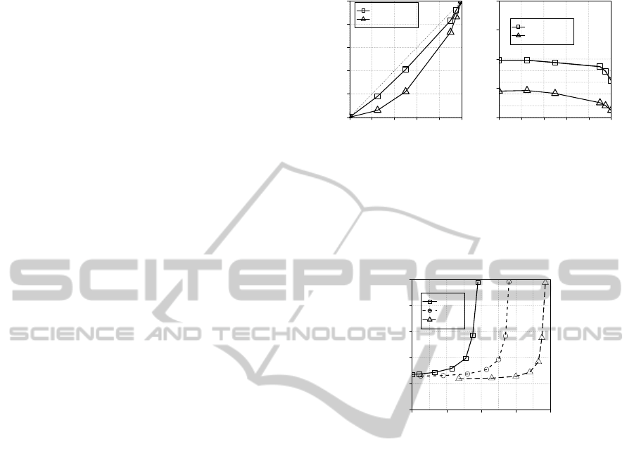
Figure 5: Measured deduplication rates and processing time
ratios.
in figure 5. The curve indicates the case of chunk
size of 8KB and 32KB. In the following experiments,
Module Deduplication Rate and the Module Process-
ing Time Ratio for other chunk sizes are estimated
based on these values.
0.0 0.2 0.4 0.6 0.8
0 1 2 3 4 5
Duplication rate
Module Processing Time ratio
128KB 64KB
32KB
16KB
8KB
4KB
2KB
r=0.4
r=0.6
r=0.8
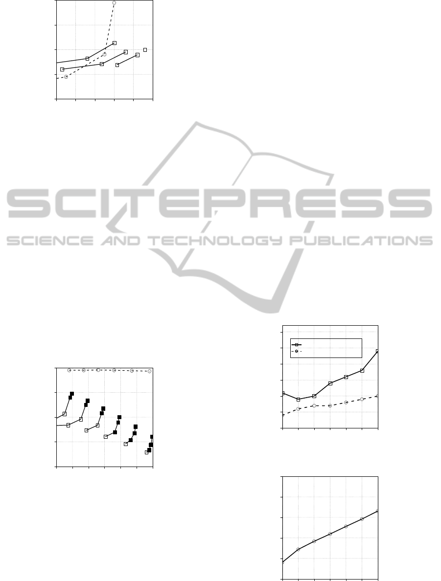
Figure 6: Single layer deduplication for r=0.4,0.6,0.8.
Figure 6 shows the correlation of a Module Pro-
cessing Time Ratio under varying chunk sizes with a
parameter of Duplication Rate ’r’. r is set to 0.4, 0.6
and 0.8. The chunk sizes are 2, 4, 8, 16, 32, 64 and
128KB. X axis means Duplication Rate, Y axis means
Module Processing Time Ratio. The smaller chunk
size is, because of their capability of more precise
deduplication, the higher the Module Deduplication
Rate is. That is asymptotic to the ideal deduplication
value of Duplication Rate itself. The figure clarifies
the heavy negative and nonlinear correlation.
5.2 Pareto Optimal Solution of Chunk
Sizes
The set of chunk sizes of a multiple layered dedu-
plication system generates a Pareto optimal solution.
Figure 7 shows the comparison of the single layer
deduplication system and the dual layered dedupli-
cation system in case of Duplication Rate equal to
0.7. X axis means SDR, Y axis means SPT. The dot-
ted line in the figure indicates the correlation over the
chunk sizes in the case of the single layer deduplica-
tion system, solid lines indicate in cases of dual lay-
TheParameterOptimizationinMultipleLayeredDeduplicationSystem
147
0.60 0.62 0.64 0.66 0.68 0.70
1 2 3 4 5
SDR
SPT
Single layer
Multiple layers
(64,8)
(64,4)
(8)
(4)
(2)
(32,8)
(32,4)
(16,8)
(16,4)
(8,4)
Figure 7: Dual layered deduplication for r=0.7.
ered deduplication system. The numbers and pairs
of numbers means the associated chunk sizes. As-
signment of smaller chunk size as the first or second
module push the SDR increasing and conversing for
the ideal number of reduction. The SPT is increasing
by using smaller chunk sizes in both systems, how-
ever the increment is defused from steep degradation
in dual layered system.
When a base of chunk size is assumed in single
layer system, the set of combinations of chunk sizes
in dual layered system can be fixed so that dual lay-
ered system provide the higher SDR and shorter SPT.
The set varies depending on which chunk size is as-
sumed as a base of the comparison. When the chunk
size of 2KB is assumed, it provides 0.66 as SDR and
4.90 as SPT. Then Set of { (16, 8), (16, 4), (8, 4) } is
Pareto optimal solution. Among the solutions, (16, 8)
is a specific to take the minimum SPT as well as (8,
4) take the maximum SDR.
0.3 0.4 0.5 0.6 0.7 0.8 0.9
1 2 3 4 5
SDR
SPT
Single layer (2KB chunk size)
Multiple layers
(Pareto optimal solution)
(8,4)
(8,4)
(32,16)
(32,16)
(16,8)
(16,4)
Figure 8: Pareto optimal solution by dual layered dedupli-
cation.
Figure 8 shows how the Pareto optimal solutions
varies depends on Duplication Rate of r. The dotted
line indicates the values of 2KB in the single layer
deduplication system as a comparison. The blacked
marks indicates subset of the Pareto optimal solution
whose elements has higher SDR and smaller SPT than
those of single layer deduplication system.
Because the choice of one of them depends on
the individual system requirement, we evaluate here
the aspects of them under changing the parameters
which are considered as a practical requirements in
the systems. The first interesting combination is the
one which provides the higher SDR to the conven-
tional single deduplication system with the minimum
SPT. The second is the one which provides the maxi-
mum SDR under predefined Backup-windows, in our
model, equivalent to TimeConstrains. The first com-
bination is called ’Minimum Time combination’ and
the second ’Maximum Rate combination’.
5.3 Improvement of System Processing
Time Ratio (SPT)
Figure 9 shows a series of L1 and L2 of Minimum
Time combination under varying Duplication Rate r.
X and Y axis means the Duplication Rate and the
chunk size, respectively, which provide the minimum
SPT. The figure indicates the aspect that the bigger the
Duplication Rate increase, the bigger the chunk sizes
are. This comes from the reason why the efficiency of
first layer reduction is higher in case of bigger chunk
size, in addition the efficiencyis more dominant while
r increases. Figure 10 shows the improvement. The
improvement increase depending on the Duplication
Rates, ex. 66% in case of 0.9 of r. This comes from
the facts that for the area of high Duplication Rate,
0.3 0.4 0.5 0.6 0.7 0.8 0.9
0 5 10 15 20 25 30
Duplication rate
Optimal chunk size [KB]
The first chunksize
The second chunksize
Figure 9: Minimum Time combination.
0.3 0.4 0.5 0.6 0.7 0.8 0.9
0 20 40 60 80 100
Duplication rate
Improvement of SPT [%]
Figure 10: Improvement of SPT.
ICEIS2013-15thInternationalConferenceonEnterpriseInformationSystems
148
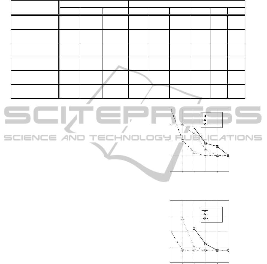
Table 2: Improvement by maximum rate chunk sizes.
Duplication Rate Multiple layered Single layer Improvement [%]
0.4 0.6 0.8 0.4 0.6 0.8 0.4 0.6 0.8
Constraints : 2 NA1 NA1 0.762 0.307 0.504 0.736 - - 3.53
(20, 10) (8) (8) (7)
Constraints : 2.5 NA1 NA1 0.791 0.330 0.533 0.748 - - 5.75
(10, 4) (6) (5) (5)
Constraints : 3 NA2 0.580 0.795 0.354 0.543 0.754 - 6.81 5.44
(12, 5) (6, 4) (4) (4) (4)
Constraints : 3.5 0.380 0.594 0.796 0.354 0.543 0.760 7.34 9.39 4.74
(9, 6) (7, 4) (5, 4) (4) (4) (4)
Constraints : 4 0.395 0.596 0.796 0.354 0.543 0.760 11.58 9.76 4.74
(8, 4) (5, 4) (5, 4) (4) (4) (4)
Constraints : 4.5 0.397 0.596 0.796 0.354 0.543 0.760 12.15 9.76 4.74
(5, 4) (5, 4) (5, 4) (4) (4) (4)
the difference of Module Deduplication Rate over the
chunk sizes decrease but the difference between the
processing time does not decrease in the same corre-
lation. The efficiency becomes bigger as the Duplica-
tion Rate increases.
In our experiments, for the area of r under 0.2,
no combination are found to achieve higher rate and
smaller time ratio. This means in case of lower Dupli-
cation Rate, the efficiency by bigger chunk size in the
first layer is eliminated due to less penalty of single
layer method.
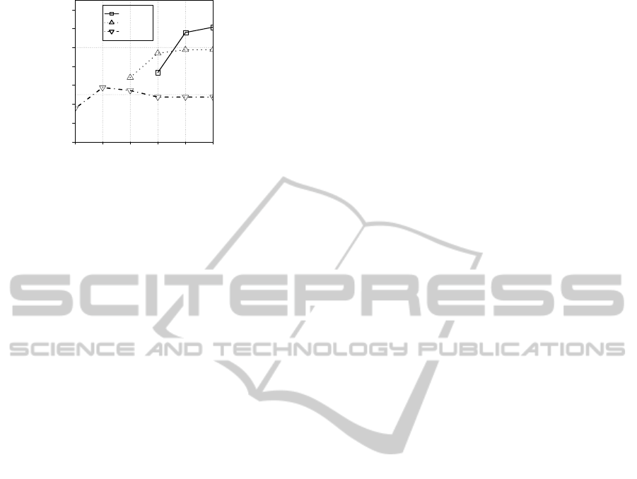
5.4 Improvement of System
Deduplication Rate (SDR)
Figure 11 shows a series of L1 of Maximum Rate
Combination under varying Duplication Rate r and
TimeConstraint. Figure 12 shows the same chart of a
series of L2. r is set to 0.4, 0.6, 0.8. TimeConstraint
is set to 2.0, 2.5, 3.0, 3.5, 4.0, 4.5. X and Y axis
means the TimeConstraint and the chunk size, re-
spectively, which provide the maximum SDR under
the TimeConstraint. The figure indicates the smaller
TimeConstraint is, the bigger the chunk sizes are.
This is the result that a small chunk size can be pro-
cessed within a small predefined time constraints. In
case of single layer deduplication system, the chunk
size which provides the maximum SDR under the
TimeConstraint is fixed as one value.
Table 2 shows Maximum Time Combination for
each value of r, 0.2, 0.4, 0.6.
The table indicates our dual layered deduplication
system can provide 30 to 40 % improvement for the
SDR and 4 to 12 % improvement for SPT. In the ta-
ble, the notation of ’NA1’ means that no combination
are found to keep the TimeConstraint, and ’NA2’ that
no combination are solved to achieve over the Dedu-
2.0 2.5 3.0 3.5 4.0 4.5
0 5 10 15 20
Time Constraint [ratio]
Optimal first chunksize [KB]
The first Chunksize
r
1
= 0.4
r
1
= 0.6
r
1
= 0.8
Figure 11: L1 of Maximum Rate combination.
2.0 2.5 3.0 3.5 4.0 4.5
0 5 10 15 20
Time Constraint [ratio]
Optimal second chunksize [KB]
The second Chunksize
r
1
= 0.4
r
1
= 0.6
r
1
= 0.8
Figure 12: L2 of Maximum Rate combination.
plication Rate of the single layer method. Figure 13
shows the improvement. The improvement increases
depending on the TimeConstraint and hits the ceiling
which is caused by the boundary of 4KB chunk size.
6 CONCLUSIONS
In this paper, we propose a new approach to improve
TheParameterOptimizationinMultipleLayeredDeduplicationSystem
149
2.0 2.5 3.0 3.5 4.0 4.5
0 2 4 6 8 10 12 14
Time Constraint [ratio]
Improvement of SDR [%]
r
1
= 0.4
r
1
= 0.6
r
1
= 0.8
Figure 13: Improvement of SDR.
the deduplication rate and the performance in backup
operation. Our system consists of a tandem type mul-
tiple layers of deduplication algorithms. The cumu-
lative deduplication rate and processing time ratio are
formularized in the comparison of conventionalsingle
layer deduplication system. Our experiments clarify
the trade-off between the maximum rate and the mini-
mum time, the Pareto optimal solution of chunk sizes,
their dependency with the file characteristics. The im-
provements are estimated as 17 to 66 % in the dedu-
plication rate and 4 to 12 % in the processing time.
REFERENCES
A. Muthitacharoen, B. Chen, and D. Mazi`eres (2001). A
low-bandwidth network file system. In Proceeding of
SIGOPS. 18th Symposium on Operating Systems Prin-
ciples., Banff, Canada.
B. Zhu, K. Li, and H. Patterson (2008). Avoiding the
disk bottleneck in the data domain deduplication
file systeme. In FASTf08: Proceedings of the 6th
USENIX Conference on File and Storage Technolo-
gies, Berkley, CA, USA. USENIX Association.
C. Dubnicki, C.Grayz, et al. (2009). Hydrastor: a scalable
secondary storage. In FAST ’09, 7th USENIX Confer-
ence on File and Storage Technologies.
C. Liu, Y. Lu, C. Shi, G. Lu, D. Lu, and D. Wang
(2008). Admad: Application-driven metadata aware
de-duplication archival storage system. In Fifth IEEE
International Workshop on Storage Network Architec-
ture and Parallel I/Os, 2008., SNAPI’08.
D. Meister and A. Brinkmann (May 2009). Multi-level
comparison of data deduplication in a backup sce-
nario. In Proceedings of SYSTOR 2009, The 2nd An-
nual International Systems and Storage Conference.
ACM.
EMC Corporation (2010). EMC Data Domain Boost Soft-
ware.
G. Wallace, F. Douglis, H. Qian, P. Shilane, S. Smaldone,
M. Chamness, and W. Hsu (2012). Characteristics of
backup workloads in production systems. In Proceed-
ings of the 10th USENIX Conference on File and Stor-
age Technologies.
J. Burrows and D. O. C. W. DC (Apritl 1995). Secure hash
standard.
M. O. Rabin (1981). Fingerprinting by random polynomi-
als. Technical report, Department of Computer Sci-
ence, Harvard University.
N. Park and D J. Lilj (2010). Characterizing datasets for
data deduplication in backup applications. In Work-
load Characterization (IISWC), 2010 IEEE Interna-
tional Symposium.
Quantum Corporation (2009). Data deduplication back-
ground: A technical white paper.
R. Rivest (1992). The MD5 Message Digest Algorithm,
RFC 1321.
U. Manber (1994). Finding similar files in a large file sys-
tem. In Proceedings of the USENIX Winter 1994 Tech-
nical Conference.
Y. Tan et al. (2010). Dam: A data ownership-aware multi-
layered de-duplication scheme. In 2010 Fifth IEEE
International Conference on Networking, Architecture
and Storage. IDC-Japan.
Y. Won, J. Ban, J. Min, L. Hur, S. Oh, and J. Lee (Sept.
2008). Efficient index lookup for de-duplication
backup system. In Modeling, Analysis and Simulation
of Computers and Telecommunication Systems, 2008.
MASCOTS 2008. IEEE International Symposium on
(Poster Presentation).
ICEIS2013-15thInternationalConferenceonEnterpriseInformationSystems
150
