Neural Networks Ensemble for Quality Monitoring

P. Thomas, M. Noyel, M. C. Suhner, P. Charpentier and A. Thomas

Centre de Recherche en Automatique de Nancy (CRAN-UMR 7039), Lorraine-Université,

CNRS Faculté des Sciences et Techniques, BP 70239, 54506 Vandoeuvre lès Nancy Cedex, France

Keywords: Neural Network, Product Quality, Neural Network Ensemble, Multivariate Quality Control, Classification,

Classifiers Ensemble.

Abstract: Product quality level is a key concept for companies' competitiveness. Different tools may be used to

improve quality such as the seven basic quality tools or experimental design. In addition, the need of

traceability leads companies to collect and store production data. Our paper aims to show that we can ensure

the required quality thanks to an "on line quality approach" based on exploitation of collected data by using

neural networks tools. A neural networks ensemble is proposed to classify quality results which can be used

in order to prevent defects occurrence. This approach is illustrated on an industrial lacquering process.

Results of the neural networks ensemble are compared with the ones obtained with the best neural network

classifier.

1 INTRODUCTION

One of the main goals in the mass customization

context is the product quality control. Statistical

process control is one of the most effective tools of

Total Quality Management (TQM). The American

Production and Inventory Control Society (APICS)

defines Total Quality Management as "A

management approach to long-term success through

customer satisfaction. TQM is based on the

participation of all members of an organization in

improving processes, goods, services, and the

culture in which they work". This definition is very

related to the definition of Just in Time (JiT) because

APICS presents JiT as “A philosophy of

manufacturing based on planned elimination of all

wastes and on continuous improvement of

productivity. One of the main elements of JiT is to

improve quality to zero defects. In the broad sense, it

applies to all forms of manufacturing”. JiT and TQM

are two major concepts related to Lean

manufacturing –LM- (Vollmann et al., 1984).

Different tools may be used to improve quality such

as the seven basic quality tools (Ishikawa chart,

check sheet, control charts, histogram, Pareto chart,

scatter diagram, stratification), or experimental

designs. These tools, along with the Taguchi

Method, are well known in the industry. Initially,

quality products was controlled a posteriori and this

a posteriori control led to reject or to downgrade a

large part of the production. Taguchi is the first to

propose to control quality before the product

origination with the set-up parameters control. this

approach based on the experimental design present

the drawback to be off-line.

In addition, the seek of traceability imposes to

companies to collect and store production data. We

propose to exploit these data in order to perform on-

line quality monitoring. The proposed approach

relies to the same philosophy as Taguchi approach.

The main goal is to set-up production parameters in

order to prevent defects occurence. This set-up is

performed on-line by taking into account the

variation in the operating range.

The first step is to extrack from data, knowledge

on the defects production. One important step of the

knowledge discovery in data processus is the

datamining step which may be performed by using

neural networks. Other tools may be used to perform

this step as fuzzy logic when expert knowledge is

available or naïve Bayes or decision tree where only

discret data are used. Neural network performs a

local search of optimum. This fact implies that the

neural network design needs to perform many

learning with different initial weights sets in order to

avoid local minimum trapping problem. These

different learning produces different classifiers more

or less performant. The simplest strategy could be to

515

Thomas P., Noyel M., Suhner M., Charpentier P. and Thomas A..

Neural Networks Ensemble for Quality Monitoring.

DOI: 10.5220/0004556505150522

In Proceedings of the 5th International Joint Conference on Computational Intelligence (NCTA-2013), pages 515-522

ISBN: 978-989-8565-77-8

 2013 SCITEPRESS (Science and Technology Publications, Lda.)

select the single, best performing classifier. Another

approach consists to use an ensemble of these

classifiers (Hansen and Salomon, 1990). This

approach based on the Condorcet's jury theorem

allows to improve the results. The second step is to

performed an on-line optimal production parameter

set-up based on the classifier ensemble results and

which may vary in function of the operating range.

The main goal of this paper is to evaluate the use

of a neural network ensemble classifier for quality

monitoring process comparing with a single neural

classifier. The design of a Taguchi experiments by

using these classifiers is also investigated in order to

find optimal tuning of controllable parameters for

considered operating point.

First, we will recall succinctly the knowledge

discovery in data process. In a second step, the

neural network structure, its learning and pruning

procedure are recalled before to present neural

network ensemble. After, the industrial application

case and the results obtained are presented before to

conclude.

2 KNOWLEDGE DISCOVERY

IN DATA FOR QUALITY

To control quality, we must understand it. So we

need to know precisely factors affecting quality.

These factors can be classified according to 6M

(Ishikawa, 1986) of the Ishikawa chart (Machine

(technology), Method (process), Material, Man

Power, Measurement (inspection), Milieu

(environment). When considering their

controllability, only 4 of the 6M must be considered:

 Environmental Factors (Environment-Milieu) such

as temperature or humidity. These factors are

generally low- or non-controllable.

 Technical Factors (Machine and Method) resulting

primarily from the machine state during

operations. They are controllable factors.

 Human Factors (Man Power) in manual

operations. They are difficult to take into account

because they sometimes vary consequently

between operators. So far, the attempts to control

human factors (establishing standards, poka yoke)

have limitations and constraints.

Knowledge on the controllability of factors is

needed in order to determine if a factor may be

tuned or considered as constraint or even as noise.

When the influential factors are correctly analyzed,

we can focus on the challenge for quality control.

The "zero defect" can be obtained in two ways:

 By optimizing the initial settings of various

factors.

 By drifts monitoring and prevention.

This paper focuses on the first way. Historically,

there are two approaches to manage quality. The

first one, and also the easiest, is to use the seven

basic quality tools (Ishikawa chart, check sheet,

control charts, histogram, Pareto chart, scatter

diagram, stratification). In this approach, the

finished parts are a posteriori controlled and

improvement propositions are performed by using

expert knowledge. In a second approach, the main

goal is to control the process and no longer the

finished parts in order to tune the technical factors

off-line by using experimental design methods.

In our approach, the production data collected

are used in order to determine the conditions of

defects apparition. To do that, a Knowledge

Discovery in Data (KDD) process may be

performed. KDD process is performed in different

steps (Patel and Panchal, 2012). We assign a letter to

each step in order to refer more easily to them later.

 Selection: obtain data from various sources (a),

 Preprocessing: cleanse data (b),

 Transformation; convert to common format,

transform to new format (c),

 Data mining: obtain desired results (d),

 Interpretation/Evaluation/Presentation: present

results to user in meaningful manner (e).

The two main steps are selection (a) and data

mining (d). Data mining which is the core part of

KDD is the process of analysing data and summarize

it into useful information. Different approaches can

be used to perform it such as artificial intelligence,

machine learning, statistics and database systems.

Data mining may perform different tasks:

 Classification: maps data into predefined group or

classes,

 Regression: maps data from an input space to an

output space,

 Clustering: groups similar data together into

clusters,

 Summarization: maps data into subsets with

associated simple descriptions,

 Link Analysis: uncovers relationships among data.

In a quality monitoring problem, the data mining

must perform a classification of data into 2 classes:

defect occurrence and no defect occurrence.

2.1 Selection (a), Preprocessing (b)

and Transformation (c) of Data

An important task in KDD process is the data

collection (a). It is possible to collect the values of

the different factors that influence quality in the

IJCCI2013-InternationalJointConferenceonComputationalIntelligence

516

same way. The availability of data is a crucial point

for the quality analysis. Ideally, the collect of data

must be automated. In the case of manual data

collection we need to increase operator awareness of

the importance of this task. Manual data collection is

often seen as a waste of time because the operator

must stop his work to write information not used

directly in production. If this task is not correctly

performed, the whole database becomes unworkable.

However, manual data collection is often inevitable,

because quality checking is often manually

performed. It is necessary to consolidate the two

types of data (production information and quality

factor values). The data must be preprocessed (b) in

order, for example, to synchronize the different

database, delete evident outliers, and digitize

qualitative data as color (c)...

2.2 Datamining (d)

The volume of data to be analyzed is often weighty

(Agard and Kusiak 2005). Companies collect and

store data for traceability reasons but they rarely use

their well of information and only as indicators for

real-time management methods (Kusiak, 2001). Data

mining is the part of Knowledge Discovery in Data

which consists in analyzing data in order to

summarize it into useful information. In our case,

data mining should perform a classification of data

into two classes: defect occurrence and no defect

occurrence. To do that, different tools may be used

such as Naïve Bayes, Decision tree, Support Vector

Machine (SVM), neural networks (NN)... Decision

tree is faster to classify data but does not work well

with noisy data (Patel and Panchal, 2012). So in the

case of industrial data, the use of this approach is not

pertinent. Naïve Bayes is dedicated to the treatment

of discrete data and the use of continuous ones needs

to perform a discretization of these data. Support

Vector Machine and Neural network both use very

close concepts which lead to very close results.

Sometimes, SVM gives better results (Meyer et al.,

2003), sometimes it is NN (Paliwal and Kumar,

2009; Hajek and Olej, 2010). This work focuses on

neural network tools which are presented in the next

section.

3 NEURAL NETWORK TOOLS

3.1 Multilayers Perceptron

We propose the use of neural networks (NN) to

model systems in order to classify quality products.

The final goal is to determine the best on-line

settings for each factor. The advantages of this

approach are:

 Exploitation of real data without carrying out

dedicated experiments as in experiments plan by

using database collected during the production.

 Simple implementation of the approach because

the neural model design is partially automated.

 On-line tuning of the quality monitoring process

by using actual production data in order to

improve and adapt the process to change.

In our approach, the neural model is performed

by using production data representatives of all the

conditions encountered in the past and so, it can

adapt itself to these changeable conditions. This

model is able to provide lower and upper limits for

each controllable factor settings based on all non-

controllable factors.

The multilayer perception (MLP) seems to be the

neural network best suited to our case. Works of

Cybenko (1989) and Funahashi (1989) have proved

that a MLP with only one hidden layer using a

sigmoïdal activation function and an output layer

can approximate all non-linear functions with the

wanted accuracy. Its structure is given by:

2101

iihhi

zg wg wx b b















(1)

where

are the n

inputs of the neural network,

w are the weights connecting the input layer to the

hidden layer,

b are the biases of the hidden

neurons,

(.) is the activation function of the hidden

neurons (here, the hyperbolic tangent),

w are the

weights connecting the hidden neurons to the output

one,

b is the bias of the output neuron g

(.) is the

activation function of the output neuron and

z is the

network output. Because of the problem is to obtain

a classification of product into two classes: defect

occurrence and no defect occurrence,

(.) being

chosen sigmoïdal.

3.2 Initialisation, Learning

and Pruning

Three steps must be performed in order to design the

neural model.

3.2.1 Initialisation

The first one is the determination of the initial set of

weights and biases. This step is important because

learning algorithm performs a local search of

NeuralNetworksEnsembleforQualityMonitoring

517

minimum. So, in order to avoid local minimum

trapping, different initial sets must be constructed

which allow beginning learning in different zones of

the criteria domain. Different initialisation

algorithms have been proposed in the literature

(Thomas and Bloch, 1997). The initialisation

algorithm used is the one proposed by Nguyen and

Widrow (1990) which allows associating a random

initialization of weights and biases to an optimal

placement in input and output spaces. This step

allows improving the diversity of the neural

classifiers which is an important notion for neural

network ensemble.

3.2.2 Learning

The second step is performed by the learning

algorithm which must fit the network output with the

data. In industrial application data are noisy and

corrupted with many outliers. In order to limit the

impact of outliers on the results, a robust Levenberg-

Marquardt algorithm is used (Thomas et al., 1999).

Levenberg–Marquard algorithm allows associating

the speed of the Hessian methods to the stability of

the gradient methods. This is performed by adding a

parameter multiplied by the identity matrix in order

to permit the inversion of the Hessian matrix even if

it is singular. The tuning of this parameter during the

learning allows the Levenberg–Marquard algorithm

to work as a gradient descent algorithm when this

parameter is large and as a Gauss–Newton algorithm

when this parameter is small. The use of a robust

criterion allows avoiding the influence of outliers

and, has a regularization effect in order to prevent

overfitting.

3.2.3 Pruning

An important issue in neural network design is the

determination of its structure. To determine it, two

approaches can be used. The first is constructive,

where the hidden neurons are added one after

another (Ma and Khorasani, 2004). The second

approach exploits a structure with too many hidden

neurons, and then prunes the least significant ones

(Setiono and Leow, 2000; Engelbrecht, 2001). We

focus on pruning approach that allows the selection

simultaneously of the input neurons and the number

of hidden neurons. The pruning phase is performed

in two steps. First, the Engelbrecht algorithm is used

which allows to quickly simplifying the structure

and second the Setiono and Leow algorithm is used

which is slower but also more efficient (Thomas and

Thomas, 2008). This step is also very important for

neural networks ensemble because it allows

improving performances of each classifier, and the

diversity of different classifiers by differentiating

there structures (pruning of inputs, hidden neurons

or weights are different for the different networks).

3.3 Neural Networks Ensemble

Neural networks ensemble is an interesting approach

to improve quality of classifier. Typically, an

ensemble classifier can be built at four different

levels (Kuncheva, 2004): Data level (Breiman,

1996), feature level (Ho, 1998), classifier level and

combination level (Kuncheva, 2002). We focus here

on classifier and combination level. The principle of

neural network ensemble is presented figure 1.

Design of ensemble neural networks consists of two

main steps: the generation of multiples classifiers

and their fusion (Dai, 2013). This leads to two

problems: how many classifiers are needed and how

to perform their fusion.

Figure 1: A neural network ensemble.

The classifier selection is a problem addressed by

many authors (Ruta and Gabris, 2005; Hernandez-

Lobato et al., 2013; Dai, 2013). Two approaches

may be used to perform it (Ruta and Gabrys, 2005):

 Static classifiers selection. The optimal selection

solution found for the validation set is fixed and

used for the classification of unseen patterns.

 Dynamic classifiers selection. The selection is

done on-line, during classification, based on

training performances and also various parameters

of the actual unlabelled pattern to classify.

In order to preserve speed of classification, we

use here a static classifiers selection. Different

selection criterions have been proposed. Individual

best performance is an universal indicator for

selection of the individual best classifiers, which is

the simplest and is reliable and robust is generally

preferred in industrial applications (Ruta and Gabrys

2005). This indicator calls minimum individual error

Network 1 Network 2 Network N

…

Combining

outputs

Input

IJCCI2013-InternationalJointConferenceonComputationalIntelligence

518

(MIE) represents the minimum error rate of the

individual classifier and promotes individual best

classifiers selection strategy:

min ( )

IE e i













(2)

where e

(i) represents the error classification of

classifier j on data i.

We use this criterion to select 100 classifiers in

order to benefit of a large classifiers set and to

obtain directly a percentage of vote representative to

the confidence of classification. Ensemble pruning

algorithm may also be used in order to optimize the

size of the classifiers ensemble (Tsoumakas et al.,

2009; Guo and Boukir, 2013).

The fusion of classifiers is generally performed

by majority vote. Kuncheva et al. (2003) have

proposed to implement limits on the majority vote

accuracy in classifier fusion. They studied the

problem of lack of independence in the classifiers

which may limit the interest of classifiers ensemble.

We implement majority vote which presents the

advantage that it could be also used as a confidence

interval on the classification results. This approach

is applied on an industrial quality control.

4 INDUSTRIAL APPLICATION

4.1 Presentation of the Process

The considered company produces high quality

lacquered panels made in MDF (Medium Density

Fiberboard) for kitchens, bathrooms, offices, stands,

shops, hotel furniture. Its main process is a robotic

lacquering workstation. Even if this workstation is

free of human factors, the production quality is

unpredictable (we cannot know if there is a risk that

products will have defects) and fluctuates (the

percentage of defects may be of 45% one day and

down to 10% the next day without changing the

settings). After a brainstorming about the factors

influencing the quality level, we were able to

classify them in three categories specified in

paragraph 2. We could imagine the potential drifts

and associate a type of defect. This preliminary work

results of expert knowledge. Only after the complete

study can we know accurately which factors affect

which defects. Thanks to a production and quality

management system, data corresponding to the

factors studied since february 2012 to september

2012 have been collected. Upstream of the robotic

lacquering workstation, experts decided to collect

factors such as load factor, number of passes, time

per table (lacquering batches), liter per table, basis

weight, number of layers, number of products and

drying time. We could add to these technical factors

environmental ones such as temperature,

atmospheric pressure and humidity. According to the

experimental design approach, we can classify these

variables into two types of factors: internal ones

(load factor, number of passes, time per table, liter

per table, basis weight, number of layers, number of

products and drying time) and external ones

(temperature, humidity, pressure). Two factors

(passes number and number of layers) are discrete

ones that can each take three states and that are

binarized (Thomas and Thomas 2009).

We have 15 inputs to apply to the neural network

which 6 are binary ones. Downstream of the

machine, we were able to detect up to 30 different

types of defects. The first works with the neural

network prediction concerning a type of defects:

"Stains on back." We have a total of 2270 data we

will split into 2 data sets for identification (1202

data) and validation (1068 data). First, learning is

achieved by exploiting 25 neurons in the hidden

layer. Pruning phase can then eliminate spurious

inputs and hidden neurons. This is done 150 times

with different initial weights sets to avoid problem

of trapping in local optimum. The 100 better

classifiers are used in the neural networks ensemble

and the performances of the neural networks

ensemble are compared with the best neural

classifier. The different initialisation sets and the

pruning phase allows to assure diversity into the

classifers set.

During the validation phase, we therefore

compare the results of the best neural classifier with

the real defects detection. For the defect "Stains on

back", we know that it occurs 127 times on the 1068

data validation set. The best neural classifier can

detect 112 defects which lead to a non-detection rate

of 11.8%. The proportion of false positive is 19.2%,

which may be partly explained by the fact that some

defects haven’t been identified out of the machine.

The quality control is performed manually. This fact

induces that some defects are not notice.

The using of neural networks ensemble on the

same validation data set gives a non-detection rate of

10.2%. The proportion of false positive is 16.4%.

These results show an improvement of 14% of the

non-detection rate and 15% on the false alarme rate.

The same work performed on a second defect (grain

on face, 477 defects on the 1068 data validation set)

allows to reduce the non detection rate from 42% to

NeuralNetworksEnsembleforQualityMonitoring

519

32% (24% of improvement) and a false alarme rate

from 21% to 16% (24% of improvement).

Another advantage of the neural networks

ensemble is that the result of the vote may be use as

a confidence interval on the classification result. As

example, for a data, a vote with 40% of defect and

60% on non defect may induces to suspect the

occurence of defect even if the classification result

leads to a non defect classification.

It is obvious that these defects are largely

explained by the archived operating conditions and

it’s possible to use neural networks ensemble

upstream of the workstation to prevent the risk of

defects. However, there are defects which cannot be

predicted with the neural networks ensemble in the

conditions described above. This is for example the

case for “knock” where you get 73% non-detection

for 11% false positives. The non predictable defects

depend certainly on other factors that we need to

determine and collect if we want to predict them. In

total, on the 30 identified defects, 7 can be partially

explained using the variables collected. For the

predictable defects, there are 2 possible approaches:

 Warning. By analyzing the inputs through the

neural networks ensemble, it becomes possible to

predict defects occurrence and report it when

conditions are met to create risk.

 Limitation. By using neural networks ensemble to

limit the input factors by upper and lower limits

and prohibit the production lot when one of the

inputs is outside these limits. If it’s a controllable

factor, operators can modify it to allow production.

Otherwise, the production lot will be rejected. It

must be scheduled later when conditions become

acceptable. To do that, factors must be classified

into controllable ones (load factor, basis weight,

drying time, liters per table), non-controllable ones

(temperature, humidity, pressure) and protocols

(number of passes, time per table, number of

layers, and number of products). The neural

networks ensemble is then used instead of the real

system to perform experiments that achieve an

entire plan without increasing the cost. The results,

however, still to be validated on the real system.

Figure 2 and 3 present the results of an entire

Taguchi plan in which 10 levels were chosen for the

3 controllable factors. In this example, for protocol

factors, we set the number of passes and layer to 1;

the time per table, and the liter of lack to their

average values; and the number of products to its

median value. We also fixed non-controllable factors

values to their average values. The effect of each

factor x

to a level A

is given classically by the mean

of all the results (defect occurence) obtained when

= A

minus the mean of the results obtained with

all the experiences. When an effect is positive, this

implies that the considered level increase the

occurence of defects, when it is negative, the

considered level reduce the occurence of defects.

The interractions between factor may be investigated

in the same way.

Figure 2 presents the results obtained with the

best neural classifier. It shows that the load factor

has a relatively small impact on the defects

occurrence. However, the increase in weight has a

significant effect. High basis weights tend to create

more defects. Drying time has also an impact

because too short drying time greatly increases the

occurrence of defects.

Figure 3 presents the same work performed by

using neural networks ensemble. Due to the

diversity of the different classifiers, the impact of

each effect are presented in the forme of an

enveloppe including the effects for all the classifiers.

We can see that the information given by the neural

networks ensemble is more complete than the one

given by the best neural classifier. If, for the load

effect, the neural networks ensemble confirms that it

has a very small impact on the defects occurence, for

the basis weight effect and dry effect, it shows that

small and large values may lead to defects

occurence.

This information can not be obtained by using

uniquely the best neural classifier. These results are

useful to tune the process parameter to their best

values under the constraint of uncontrollable factors

as meteorological ones.

As example, with the operating range considered

here, the set-up of the basis weight may be tuned

between 90 and 190 when the tuning of dry time

may be tuned between 400 and 1100 in order to limit

the risk of defects occurence.In order to obtain the

same results by using an experiments plan, we need

to use 5 modalities for drying time and basis weight

and 2 for the load factor that lead to many

experiments even using Taguchi plan. These

preliminary results need to be confirmed by taking

into account the variation of non-controllable factors

(temperature, pressure and humidity) and validating

the results on the real system.

IJCCI2013-InternationalJointConferenceonComputationalIntelligence

520

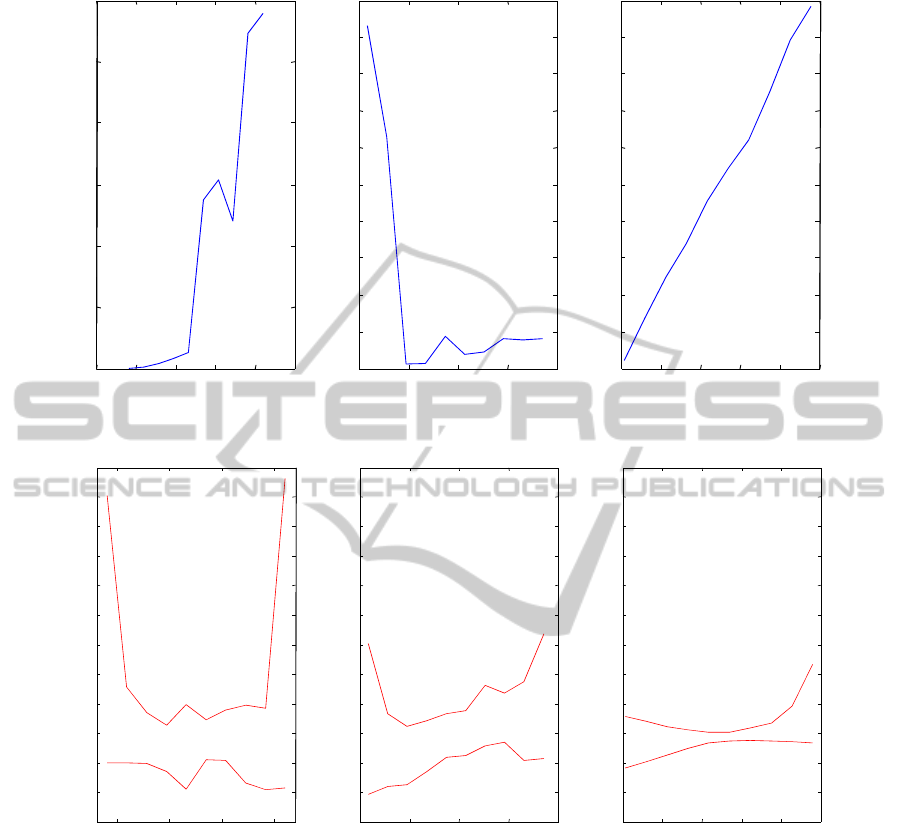
Figure 2: Experiment plan results by using best NN classifier.

Figure 3: Experiment plan results by using neural networks ensemble.

5 CONCLUSIONS

This paper presents neural networks ensemble for

quality monitoring comparing to single neural

classifier. The approach is applied and tested on an

industrial application. The results show that a neural

networks ensemble allows improving greatly the

classification performance. We show that neural

networks ensemble, as single classifier, allows

performing Taguchi experiments in order to find the

best tuning of parameters in order to avoid defects

occurrence. Due to diversity of classifier, the results

of Taguchi experiments obtained by using neural

networks ensemble are more complete and useful.

Two ways of improvement must be performed in

the future works. The first one is to use pruning

ensemble algorithm in order to optimize the size of

the ensemble in function of the results. The second

one is to improve the diversity of classifiers by using

other classifiers tools as support vector machines,

fuzzy logic or genetic algorithms.

REFERENCES

Agard, B., Kusiak, A., 2005. Exploration des bases de

0 50 100 150 200 250

-0.02

-0.01

0.01

0.02

0.03

0.04

Levels for basis weight factor

0 500 1000 1500 2000

-0.02

-0.01

0.01

0.02

0.03

0.04

0.05

0.06

0.08

Level s for dry time factor

0 1 2 3 4 5

-5

-4

-3

-2

-1

x 10

-3

Levels for load factor

effect

on defects

occurrence

effect

on defects

occurrence

effect

on defects

occurrence

50 100 150 200

-0.1

-0.05

0.05

0.1

0.15

0.2

0.25

0.3

0.35

0.4

Levels for basis weight factor

0 500 1000 1500 2000

-0.1

-0.05

0.05

0.1

0.15

0.2

0.25

0.3

0.35

0.4

Levels for dry time factor

0 1 2 3 4 5

-0.1

-0.05

0.05

0.1

0.15

0.2

0.25

0.3

0.35

0.4

Levels for load factor

Effect on

defect

occurrence

Effect on

defect

occurrence

Effect on

defect

occurrence

NeuralNetworksEnsembleforQualityMonitoring

521

données industrielles à l’aide du datamining –

Perspectives. 9

ème

colloque national AIP PRIMECA.

Breiman, L., 1996. Bagging predictors. Machine Learning,

24, 2, 123-140.

Cybenko, G., 1989. Approximation by superposition of a

sigmoïdal function. Math. Control Systems Signals, 2,

4, 303-314.

Dai, Q., 2013. A competitive ensemble pruning approach

based on cross-validation technique. Knowledge-

Based Systems. 37, 394-414.

Engelbrecht, A. P., 2001. A new pruning heurisitc based

on variance analysis of sensitivity information. IEEE

trasanctions on Neural Networks, 1386-1399.

Funahashi, K., 1989. On the approximate realisation of

continuous mapping by neural networks. Neural

Networks, 2, 183-192.

Guo, L., Boukir, S., 2013. Margin-based ordered

aggregation for ensemble pruning. Pattern

Recognition Letters, 34, 603-609.

Hajek, P., Olej, V., 2010. Municipal revenue prediction by

ensembles of neural networks and support vector

machines. WSEAS Transactions on Computers, 9,

1255-1264.

Hansen, L. K., Salomon, P., 1990. Neural network

ensembles. IEEE Transactions on Pattern Analysis

and Machine Intelligence. 12, 10, 993-1001.

Hernandez-Lobato, D., Martinez-Munoz, G., Suarez, A.,

2013. How large should ensembles of classifiers be?

Pattern Recognition. 46, 1323-1336.

Ho, T., 1998. The random subspace method for

constructing decision forests. IEEE Transactions on

Pattern Analysis and Machine Intelligence. 20, 8, 832-

844.

Ishikawa, K., 1986. Guide to quality control. Asian

Productivity Organization.

Kuncheva, L. I., 2002. Switching between selection and

fusion in combining classifiers: An experiment. IEEE

Transactions on Systems, Man and Cybernetics, part

B: Cybernetics. 32, 2, 146-156.

Kuncheva, L. I., 2004. Combining pattern classifiers:

Methods and algorithms. Wiley-Intersciences.

Kuncheva, L. I., Whitaker, C. J., Shipp, C. A., 2003.

Limits on the majority vote accuracy in classifier

fusion. Pattern Analysis and Applications. 6, 22-31.

Kusiak, A., 2001. Rough set theory: a data mining tool for

semiconductor manufacturing. Electronics Packaging

Manufacturing, IEEE Transactions on, 24, 44-50.

Ma, L., Khorasani, K., 2004. New training strategies for

constructive neural networks with application to

regression problems. Neural Network, 589-609.

Meyer, D., Leisch, F., Hornik, K., 2003. The support

vector machine under test. Neurocomputing, 55, 169-

186.

Nguyen, D., Widrow, B., 1990. Improving the learning

speed of 2-layer neural networks by choosing initial

values of the adaptative weights. Proc. of the Int. Joint

Conference on Neural Networks IJCNN'90, 3, 21-26.

Paliwal, M., Kumar, U. A., 2009. Neural networks and

statistical techniques: A review of applications. Expert

Systems with Applications, 36, 2-17.

Patel, M. C., Panchal, M., 2012. A review on ensemble of

diverse artificial neural networks. Int. J. of Advanced

Research in Computer Engineering and Technology,

1, 10, 63-70.

Ruta, D., Gabrys, B., 2005. Classifier selection for

majority voting. Information Fusion. 6, 63-81.

Setiono, R., Leow, W.K., 2000. Pruned neural networks

for regression. 6th Pacific RIM Int. Conf. on Artificial

Intelligence PRICAI’00, Melbourne, Australia, 500-

509.

Thomas, P., Bloch, G., 1997. Initialization of one hidden

layer feedforward neural networks for non-linear

system identification. 15

IMACS World Congress on

Scientific Computation, Modelling and Applied

Mathematics WC'97, 4, 295-300.

Thomas, P., Bloch, G., Sirou, F., Eustache, V., 1999.

Neural modeling of an induction furnace using robust

learning criteria. J. of Integrated Computer Aided

Engineering, 6, 1, 5-23.

Thomas, P., Thomas, A., 2008. Elagage d'un perceptron

multicouches : utilisation de l'analyse de la variance de

la sensibilité des paramètres. 5

ème

Conférence

Internationale Francophone d'Automatique CIFA'08.

Bucarest, Roumanie.

Thomas, P., Thomas, A., 2009. How deals with discrete

data for the reduction of simulation models using

neural network. 13

IFAC Symp. On Information

Control Problems in Manufacturing INCOM’09,

Moscow, Russia, june3-5, 1177-1182.

Tsoumakas, G., Patalas, I., Vlahavas, I., 2009. An

ensemble pruning primer. in Applications of

supervised and unsupervised ensemble methods O.

Okun, G. Valentini Ed. Studies in Computational

Intelligence, Springer.

Vollmann, T. E., Berry, W.L. and Whybark, C. D., 1984.

Manufacturing Planning and Control Systems, Dow

Jones-Irwin.

IJCCI2013-InternationalJointConferenceonComputationalIntelligence

522