A Methodology for the Design of Fuzzy Fractional PID Controllers
Ramiro S. Barbosa and Isabel S. Jesus
GECAD - Knowledge Engineering and Decision Support Research Center, ISEP/IPP - School of Engineering,
Polytechnic Institute of Porto,
Rua Dr. Antonio Bernardino de Almeida, 431, Porto, Portugal
Keywords:
Fuzzy Control, PID Controller, Fractional Calculus, Fractional PID Control, Fuzzy Fractional PID Control.
Abstract:
This paper proposes two novel fuzzy fractional PID structures. The tuning of the fuzzy fractional controllers
is based on the prior knowledge of fractional-order control tuning rules. The digital implementation of these
controllers is also investigated. The effectiveness and robustness of the proposed tuning methodology is illus-
trated through its application on a fractional-order plant. The simulations results show that the control system
performance is better than that of conventional fractional PID control.
1 INTRODUCTION
In recent years, the fractional-order PID (FO-PID)
controllers have been a fruitful field of research (Pod-
lubny, 1999a; Podlubny, 1999b). However, no effec-
tive and simple tuning rules still exist for these con-
trollers as those given for the integer PID controllers
(Astrom and Hagglund, 1995). It is well known that
the FO-PID extends the capabilities of the classical
counterpart and, thus, have a wider domain of appli-
cation, such as in suspension systems, robotics, sig-
nal processing, control and diffusion (Oldham and
Spanier, 1974; Podlubny, 1999a; Podlubny, 1999b).
On the other hand, the fuzzy logic controllers (FLC)
have also been successfully applied in the control of
many physical systems, particularly those with un-
certainty, unmodelled, disturbed and/or nonlinear dy-
namics (Lee, 1990; Li and Gatland, 1996; Carvajal
et al., 2000).
In this paper, we combine the features of fuzzy
controllers with those of fractional controllers of PID-
type. The resulting fuzzy fractional PID (FF-PID)
controller is investigated in terms of its digital imple-
mentation and robustness. The combined advantages
of the two controllers results in a better controller with
superior robustness and wider domain of application.
The tuning methodology of these controllers is based
on the prior knowledge of fractional-order control.
First, a fractional-order controller is built and tuned
(or used one already implemented). Then, we replace
it with a linear fuzzy fractional controller displaying
exactly the same step response. After, we make the
controller nonlinear and fine tune it in order to get
better control of the system. The fuzzy fractional con-
troller will give, at least, the same performance of its
linear counterpart.
The paper is organized as follows. Section 2
presents the basic ideas of continuous and discrete
fractional PID controllers. Section 3 outlines a pro-
cedure for the design of FF-PID controllers. In sec-
tion 4, we test the proposed fuzzy fractional con-
trollers and assess their applicability and robustness
on a fractional-order plant. Finally, section 5 draws
the main conclusions and addresses perspectives to
future developments.
2 FRACTIONAL PID
CONTROLLERS
The fractional-order controller of PID-type, usually
named PI
λ
D
µ
controller, may be given as (Podlubny,
1999b; Barbosa et al., 2010):
C(s) =
U (s)
E (s)
= K
p
+
K
i
s
λ
+ K
d
s
µ
(1)
where K
p
, K
i
and K
d
are the proportional, inte-
gral and derivative gains, and usually the fractional
orders (λ, µ) ∈ [0, 1]. Clearly, taking (λ, µ) ≡
{(1, 1), (1, 0), (0, 1), (0, 0)} we get the classical
{PID, PI, PD, P}-controllers, respectively. The
PI
λ
D
µ
-controller is more flexible and gives the possi-
bility of adjusting more carefully the dynamical pro-
prieties of a control system (Podlubny, 1999b).
276
S. Barbosa R. and S. Jesus I..
A Methodology for the Design of Fuzzy Fractional PID Controllers.
DOI: 10.5220/0004586702760281
In Proceedings of the 10th International Conference on Informatics in Control, Automation and Robotics (ICINCO-2013), pages 276-281
ISBN: 978-989-8565-70-9
Copyright
c
 2013 SCITEPRESS (Science and Technology Publications, Lda.)

The time domain equation of the PI
λ
D
µ
controller
is:
u(t) = K
p
e(t)+ K
i
D
−λ
e(t)+ K
d
D
µ
e(t) (2)
where D
(∗)
(≡
0
D
α
t
) denotes the differential operator
of integration and differentiation (differintegral) to a
fractional-order α = {−λ, µ} ∈ ℜ.
The two most commonly used definitions for the
differintegral are the Riemann-Liouville definition
and the Gr¨unwald-Letnikov definition. For our pur-
pose we use the Gr¨unwald-Letnikov definition, which
can be written as (α ∈ ℜ):
D
α
f (t) = lim
h→0
1
h
α
[t
/
h]
∑
j=0
(−1)
j

α
j

f (t − jh) (3a)

α
j

=
Γ(α + 1)
Γ( j+ 1)Γ(α− j + 1)
(3b)
where f(t) is the applied function, Γ(·) is the Gamma
function, h is the time increment, and [·] means the
integer part.
From a control and signal processing perspective,
approach (3) seems to be the most useful and intu-
itive, particularly for a discrete-time implementation
(Barbosa et al., 2006; Machado, 1997). In fact, using
(3), a discrete fractional PI
λ
D
µ
control equation can
be obtained from (2) as (h ≈ T, T is the sampling
period):
u(k) = K
p
e(k) + K
i
D
−λ
e(k) + K
d
D
µ
e(k) (4)
with
D
α
e(k) ≈
1
T
α
k
∑
j=0
(−1)
j

α
j

e(k − j) (5)
The difference control equation (4) is then given
by:
u(k) = K
p
e(k) +
K
i
T
−λ
k
∑
j=0
(−1)
j

−λ
j

e(k − j)
+
K
d
T
µ
k
∑
j=0
(−1)
j

µ
j

e(k − j) (6)
Eq. (6) shows that the current value of control sig-
nal u(k) depends on all previous values of error e(k),
making the computation too heavy as time increases
and so unsuitable for a practical implementation of
these algorithms. This fact illustrates the global char-
acter (i.e., unlimited memory) of the fractional-order
operators. For practical implementation of fractional
integral and derivative (5) we often apply the short
memory principle (Podlubny, 1999a), resulting in ex-
pression:
u(k) = K
p
e(k) +
K
i
T
−λ
k
∑
j=v
c
(−λ)
j
e(k − j)
+
K
d
T
µ
k
∑
j=v
c
(µ)
j
e(k − j) (7)
where v = 0 for k < L

T or v = k−L

T for k > L

T;
L is the memory length and c
(α)
j
= (−1)
j

α
j

are
the binomial coefficients which may be calculated re-
cursively as:
c
(α)
0
= 1; c
(α)
j
=

1−
1+ α
j

c
(α)
j−1
, j = 1, 2, ···
(8)
Note that (7) is given in the form of a FIR filter.
Other discrete-time approximations in the form of IIR
filters are also possible (Vinagre et al., 2003; Barbosa
et al., 2006; Chen et al., 2004).
3 DESIGN OF FUZZY
FRACTIONAL PID
CONTROLLERS
Despite of variety of possible fuzzy controller struc-
tures, the controller is usually arranged in cascade
with the system being controlled. This type of ar-
rangement is shown in Fig. 1 and will be used in this
study.
The main idea here is to explore the fact that the
FLC, under certain conditions, is equivalent to a PID
controller (Mizumoto, 1995; Li and Gatland, 1996;
Jantzen, 2007). In a certain sense, the fuzzy PID con-
trollers are a special case of the more general FF-PID
controllers, in which are involved two extra tuning
parameters: the fractional orders (λ, µ) of controller
equation (4).
The basic form of a fuzzy controller is illustrated
in Fig. 2 (Passino and Yurkovich, 1998). In gen-
eral, the mapping between the inputs and the outputs
−
+
G(s)
Fuzzy
Fractional
Controller
r(t) y(t)
u(t)
e(t)
l(t)
+
+
Figure 1: Fuzzy fractional PID controlled system.
AMethodologyfortheDesignofFuzzyFractionalPIDControllers
277

Rule Base
Fuzzy
inference
Fuzzification
Defuzzification
Input Output
Figure 2: Structure of a fuzzy controller.
of a fuzzy system is nonlinear (Galichet and Foulloy,
1995; Jantzen, 2007). However, it is possible to con-
struct a rule base with a linear input-output mapping
(Mizumoto, 1995; Jantzen, 2007). For that, the fol-
lowing conditions must be fulfilled:
• Use triangular input sets that cross at the member-
ship value 0.5;
• The rule base must be complete AND combina-
tion (cartesian product) of all input families;
• Use the algebraic product (*) for the AND con-
nective;
• Use output singletons, positioned at the sum of the
peak positions of the input sets;
• Use sum-accumulation and centre of gravity for
singletons (COGS) defuzzification.
It seems reasonable to start with the design of
a conventional integer/fractional PID controller and
from there to proceed to a fuzzy control design. In
this way, the linear fuzzy controller may be used in a
design procedure based on integer/fractionalPID con-
trol, as follows (Jantzen, 2007; Barbosa et al., 2010;
Barbosa, 2010):
1. Build and tune an integer/fractional PID con-
troller;
2. Replace it with an equivalent linear fuzzy con-
troller;
3. Make the fuzzy controller nonlinear;
4. Fine-tune it.
With the above procedure, the design of fuzzy
fractional PID controllers will be greatly simplified,
particularly if the controller was already implemented
and it is desirable to enhance its performance. More-
over, this new type of controllers extends the poten-
tialities of both fuzzy and fractional controllers and
performs, at least, as well as its linear fractional coun-
terpart (Jantzen, 2007; Barbosa et al., 2010; Barbosa,
2010).
3.1 Fuzzy Fractional PD Controller
The time-domain equation of a fractional PD
µ
-
controller is given by (K
i
= 0 in (2)):
u(t) = K
p
e(t) + K
d
D
µ
e(t) (9)
The corresponding discrete-time fractional PD
µ
-
controller is:
u(k) = K
p
e(k) + K
d
D
µ
e(k) (10)
Fig. 3 illustrates the block diagram of the fuzzy
fractional PD
µ
(FF-PD
µ
) controller. As can be seen,
the controller acts on the error, E = K
e
e(k), and on
the fractional change of error, FE = K
fe
D
µ
e(k). The
control signal is U = K
u
u. The controller has three
tuning gains, K
e
and K
fe
, corresponding to the inputs
and K
u
to the output.
The control signalU is generally a nonlinear func-
tion of E and FE:
U = f(E, FE)K
u
= f (K
e
e, K
fe
D
µ
e)K
u
(11)
With a proper choice of design, a linear approxi-
mation can be obtained as:
f (K
e
e(k), K
fe
D
µ
e(k)) ≈ K
e
e(k)+K
fe
D
µ
e(k) (12)
and
U (k) = (K
e
e(k) + K
fe
D
µ
e(k))K
u
= K
e
K
u
e(k) + K
fe
K
u
D
µ
e(k) (13)
Comparing (13) with (10), it yields the relation for
the gains of the two controllers:
K
e
K
u
= K
p
K
fe
K
u
= K
d
(14)
The linear FF-PD
µ
-controller provides all the
advantages of the conventional fractional PD
µ
-
controller.
For an equivalent linear FF-PD
µ
-controller, the
conclusion universe should be the sum of the premise
universes and the input-output mapping should be lin-
ear. Table 1 lists a linear rule base for the FF-PD
µ
controller composed of four rules. There are only
two fuzzy labels (Negative and Positive) used for the
fuzzy input variables and three fuzzy labels (Negative,
Zero and Positive) for the fuzzy output variable. This
rule base should satisfy conditions mentioned above
in order to provide a linear mapping.
FF-PD
µ
Rule base
E
FE
Uu
e
u
K
fe
K
e
K
µ
D
Figure 3: Fuzzy fractional PD
µ
-controller.
ICINCO2013-10thInternationalConferenceonInformaticsinControl,AutomationandRobotics
278

Table 1: Rule base for the FF-PD
µ
controller.
Rule 1 If E is N and FE is N then u is N
Rule 2 If E is N and FE is P then u is Z
Rule 3 If E is P and FE is N then u is Z
Rule 4 If E is P and FE is P then u is P
Scaling the input gains may be necessary to pre-
serve the linearity of the fuzzy controller. However,
that should be made without affectingthe tuning (Bar-
bosa et al., 2010; Barbosa, 2010). This scaling has
some advantages, as it will avoid saturation and will
provide a simpler design, since the universes ranges
of inputs and outputs are normalized to a prescribed
interval, say percentage of full scale [−100, 100].
3.2 Fuzzy Fractional PID Controller
The inclusion of an integral action is necessary when-
ever the closed-loop system exhibits a steady-state er-
ror. The fuzzy fractional PD
µ
+I
λ
(FF-PD
µ
+I
λ
) con-
troller combine the fractional-order integral action
with a fuzzy PD
µ
-controller, as illustrated in Fig. 4.
FF-PD
µ
Rule base
E
FE
U
u
e
u
K
fe
K
e
K
µ
D
fie
K
FIE
+
+
λ−
D
Figure 4: Fuzzy fractional PD
µ
+ I
λ
controller.
The control signalU is generally a nonlinear func-
tion of error E, fractional change of error FE, and
fractional integral of error FIE:
U = ( f (E, FE) + FIE) K
u
=

f (K
e
e(k) + K
fe
D
µ
e(k)) + K
fie
D
−λ
e(k)

K
u
(15)
Adopting the linear approximation (12) yields the
control action:
U (k) ≈

K
e
e(k) + K
fe
D
µ
e(k) + K
fie
D
−λ
e(k)

K
u
= K
u
K
e
e(k) + K
u
K
fe
D
µ
e(k) + K
u
K
fie
D
−λ
e(k) (16)
Comparing (16) with the discrete fractional PI
λ
D
µ
-
controller (4), it yields the relation for the gains of
the two controllers:
K
e
K
u
= K
p
K
fie
K
u
= K
i
K
fe
K
u
= K
d
(17)
The linear FF-PD
µ
+I
λ
controller provides all the
advantages of the conventional fractional PI
λ
D
µ
-
controller.
4 ILLUSTRATIVE EXAMPLE
Many real dynamical processes are modeled by
fractional-order transfer functions (Podlubny, 1999a;
Oldham and Spanier, 1974). Here we consider
the fractional-order plant model given in (Podlubny,
1999b):
G(s) =
1
0.8s
2.2
+ 0.5s
0.9
+ 1
(18)
An integer-order PD controller and a fractional-
order PD
µ
-controller were designed in (Podlubny,
1999b):
C
PD
(s) = 20.5+ 2.7343s (19)
C
PD
µ
(s) = 20.5+ 3.7343s
1.15
(20)
Fig. 5 shows the unit-step response of the closed-
loop fractional-order system with the conventional
PD-controller and with the PD
µ
-controller. The com-
parison shows that for satisfactory feedback con-
trol of the fractional-order system is better to use a
fractional-order controller. Note, however, that the
control system presents a steady-state error, since no
integral action is employed.
Let us now design an equivalent linear FF-PD
µ
controller. By configuring the fuzzy inference system
(FIS) and selecting three scaling factors, we obtain a
FF-PD
µ
-controller that reproduces the exact control
performance as the fractional PD
µ
-controller. We first
fix K
e
= 100, since the error universe is chosen to be
0 1 2 3 4 5 6
0
0.2
0.4
0.6
0.8
1
1.2
1.4
1.6
Time [s]
Plant output
PD−controller
PD
µ
−controller
Figure 5: Unit-step responses of the fractional-order control
system with the PD and PD
µ
-controllers.
AMethodologyfortheDesignofFuzzyFractionalPIDControllers
279

−100
0
100
−100
0
100
−200
0
200
E
FE
u
−100 0 100
0
0.2
0.4
0.6
0.8
1
Input family: Neg and Pos
Degree of membership
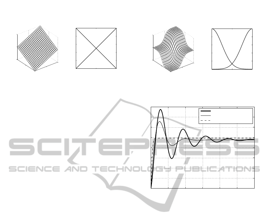
Figure 6: Linear surface with the corresponding input fam-
ilies.
percentage of full scale [−100, 100], and the maxi-
mum error to a unit step is 1. The values of K
fe
and
K
u
are obtained using expressions (14). Fig. 6 shows
the input families and the linear control surface ob-
tained by using the rule base of Table 1 while satis-
fying conditions outlined in section 3. Note that this
result represents the step 2 – replace the conventional
controller with an equivalent linear fuzzy controller –
of the design procedure. In order to enhance the per-
formance of the control system we proceed to step 3
and 4 of the design – make the fuzzy controller non-
linear and fine-tune it.
Thus, after verifying that the linear FF-PD
µ
-
controller is properly designed, we may adjust the FIS
settings such as its style, membership functions and
rule base to obtain a desired nonlinear control sur-
face. In our example, we choose Gaussian member-
ship functions for the inputs, as illustrated in Fig. 7
with the corresponding nonlinear control surface.
In Fig. 8, the comparison of the unit-step response
of the closed-loop system with plant model (18) con-
trolled by the linear PD and FF-PD
µ
-controllers, and
with the nonlinear FF-PD
µ
-controller is given. The
simulation parameters are: absolute memory compu-
tation of approximation (5), fractional-order µ=1.15,
scale factor M = 0.4 and T = 0.05 s. As can be seen,
making the controller nonlinear improved the control
system performance, namely the overshoot, rise time,
settling time, and steady-state error, when compared
with the linear fuzzy controller. The fuzzy fractional
controller provides greater flexibility than the frac-
tional controller and can be used to better adjust the
dynamical properties of a control system.
Now, let us consider the FF-PD
µ
+I
λ
-controller. In
order to test the robustness of the fuzzy controller, we
introduce a load disturbance of amplitude l = 2 after
7 seconds in system of Fig. 1. We use the same (K
p
,
K
d
) parameters of the linear FF-PD
µ
-controller and
tuned the (K
i
, λ) for a satisfactory control response.
The final tuned parameters are (K
i
, λ) = (10, −0.8).
With K
e
= 100, and using (17) we obtain K
fe
, K
u
, and
K
fie
of the fuzzy controller.
−100
0
100
−100
0
100
−200
0
200
E
FE
u
−100 0 100
0
0.2
0.4
0.6
0.8
1
Input family: Neg and Pos
Degree of membership
Figure 7: Nonlinear control surface with the corresponding
input families.
0 1 2 3 4 5 6
0
0.2
0.4
0.6
0.8
1
1.2
1.4
1.6
Time [s]
Plant output
PD−controller
FF−PD
µ
−controller
Nonlinear FF−PD
µ
−controller
Figure 8: Unit-step responses of the fractional control sys-
tem with the linear PD and FF-PD
µ
-controllers, and with
the nonlinear FF-PD
µ
-controller.
In this experiment, the simulation parameters are:
absolute memory computation of approximation (5),
scale factor M = 0.1 and T = 0.05 s. Fig. 9 shows the
step and load responses of closed-loop system with
FF-PD
µ
+I
λ
controller, (µ, λ)=(1.15, −0.8), for the lin-
ear and nonlinear control surfaces. We observe the
better response of the fuzzy controller to the reference
and disturbance inputs with the nonlinear rule base
compared to their linear counterpart. Once more, we
demonstrate the robustness and effectiveness of this
type of controller.
5 CONCLUSIONS
This paper introduced two novel fuzzy fractional PID
structures: the FF-PD
µ
and FF-PD
µ
+I
λ
controllers. It
was demonstrated that these controllers are equiva-
lent to the conventional fractional PD and PID con-
trollers by using a linear input-output mapping of the
rule base of the fuzzy fractional controller. Moreover,
by making the controller nonlinear, the performance
of the control system proves to be, in most systems,
better than its linear counterpart. A methodology for
ICINCO2013-10thInternationalConferenceonInformaticsinControl,AutomationandRobotics
280

0 5 10 15 20
0
0.2
0.4
0.6
0.8
1
1.2
1.4
1.6
Time [s]
Plant output
Linear FF−PD
µ
+I
λ
controller
Nonlinear FF−PD
µ
+I
λ
controller
Figure 9: Unit-step and load responses of the fractional con-
trol system with the linear and nonlinear FF-PD
µ
+I
λ
con-
trollers.
tuning the nonlinear fuzzy fractional PID controllers
is also presented. This methodology is simple and
effective and can be used to replace an existent frac-
tional/integer PID controller in order to get better per-
formance of the control system. In this perspective,
future research on this topic includes the application
of the proposed fuzzy fractional PID controllers and
tuning methodology in other types of linear and non-
linear plants of integer and/or fractional-order. We
expect that the incorporation of fuzzy reasoning into
fractional-order controllers will increase the applica-
bility of these controllers.
ACKNOWLEDGEMENTS
This work is supported by FEDER Funds through
the ”Programa Operacional Factores de Competitivi-
dade - COMPETE” program and by National Funds
through FCT ”Fundac¸˜ao para a Ciˆencia e a Tecnolo-
gia”.
REFERENCES
Astrom, K. J. and Hagglund, T. (1995). PID Controllers:
Theory, Design, and Tuning. Instrument Society of
America, USA.
Barbosa, R. S., , Jesus, I. S., and Silva, M. F. (2010). Fuzzy
reasoning in fractional-order PD controllers. In Pro-
ceedings of AIC’10, 10th WSEAS International Con-
ference on Applied Informatics and Communications,
pages 252–257, August 20-22, Taipei, Taiwan.
Barbosa, R. S. (2010). On linear fuzzy fractional pd and
pd+i controllers. In Proceedings of FDA’10, 4th IFAC
Workshop Fractional Differentiation and its Applica-
tions, pages 1–6, October 18-20, Badajoz, Spain.
Barbosa, R. S., Machado, J. A. T., and Silva, M. F. (2006).
Time domain design of fractional differintegrators
uing least-squares. Signal Processing, 86:2567–2581.
Carvajal, J., Chen, G., and Ogmen, H. (2000). Fuzzy
PID controller: Design, performance evaluation, and
stability analysis. Journal of Information Science,
123:249–270.
Chen, Y. Q., Vinagre, B. M., and Podlubny, I. (2004).
Continued fraction expansion approaches to discretiz-
ing fractional order derivatives-an expository review.
Nonlinear Dynamics, 38:155–170.
Galichet, S. and Foulloy, L. (1995). Fuzzy controllers: Syn-
thesis and equivalences. IEEE Transactions on Fuzzy
Systems, 3(2):140–148.
Jantzen, J. (2007). Foundations of Fuzzy Control. Wiley
and Sons, Chichester, England.
Lee, C. C. (1990). Fuzzy logic in control systems: fuzzy
logic controller-Part I and II. IEEE Transactions on
System Man, and Cybernetics-Part B: Cybernetics,
20(2):404–435.
Li, H.-H. and Gatland, H. B. (1996). Conventional fuzzy
control and its enhancement. IEEE Transactions on
System Man, and Cybernetics-Part B: Cybernetics,
26(5):791–797.
Machado, J. A. T. (1997). Analysis and design of fractional-
order digital control systems. SAMS Journal of Sys-
tems Analysis, Modelling and Simulation, 27:107–
122.
Mizumoto, M. (1995). Realization of PID control by fuzzy
control methods. Fuzzy Sets and Systems, 70:171–
182.
Oldham, K. B. and Spanier, J. (1974). The Fractional Cal-
culus. Academic Press, New York.
Passino, K. M. and Yurkovich, S. (1998). Fuzzy Control.
Addison-Wesley, Menlo Park, California.
Podlubny, I. (1999a). Fractional Differential Equations.
Academic Press, San Diego.
Podlubny, I. (1999b). Fractional-order systems and PI
λ
D
µ
-
controllers. IEEE Transactions on Automatic Control,
44(1):208–214.
Vinagre, B. M., Chen, Y. Q., and Petras, I. (2003). Two di-
rect tustin discretization methods for fractional-order
differentiator/integrator. Journal of the Franklin Insti-
tute, 340:349–362.
AMethodologyfortheDesignofFuzzyFractionalPIDControllers
281