
Global Camera Parameterization for Bundle Adjustment
ˇ
Cenˇek Albl and Tom´aˇs Pajdla
Department of Cybernetics, CTU in Prague, Prague, Czech Republic
Keywords:
Bundle Adjustment, Structure From Motion, Perspective Camera, Camera Parameterization, Quaternion.
Abstract:
Bundle adjustment is an important optimization technique in computer vision. It is a key part of Structure from
Motion computation. An important problem in Bundle Adjustment is to choose a proper parameterization of
cameras, especially their orientations. In this paper we propose a new parameterization of a perspective camera
based on quaternions, with no redundancy in dimensionality and no constraints on the rotations. We conducted
extensive experiments comparing this parameterization to four other widely used parameterizations. The
proposed parameterization is non-redundant, global, and achieving the same performance in all investigated
parameters. It is a viable and practical choice for Bundle Adjustment.
1 INTRODUCTION
Structure from motion (SfM) reconstruction received
a lot of attention resulting in many practical appli-
cations such as Photosynth (Microsoft, 2008) and
Bundler (Snavely, 2011). Current research aims
at providing more precise reconstruction as well as
the ability to handle larger datasets (Agarwal et al.,
2010), (Crandall et al., 2011).
Bundle Adjustment (BA) (Triggs et al., 2000) is
an important part of SfM as it optimizes the result-
ing estimates of 3D point coordinates and the po-
sition, orientation, and calibration of cameras (Fig-
ure 1). Detailed analysis of BA optimization methods,
parameterizations, error modeling and constraints has
been given in (Triggs et al., 2000). An efficient
and comprehensive algorithm that utilizes the spar-
sity of BA has been developed by Lourakis and Ar-
gyros (Lourakis and Argyros, 2009) and the code was
made freely available. This algorithm has been fur-
ther used in (Snavely, 2011) to build a full struc-
ture from motion pipeline. An extended version
of (Lourakis and Argyros, 2009) has been developed
in (Konolige, 2010) utilizing the sparsity even further
in order to reduce computation time. Recently, the
performance of BA on large datasets has been scru-
tinized (Agarwal et al., 2010). The use of conjugate
gradients and its effect on performance has been in-
vestigated in (Byr¨od and
˚
Astr¨om, 2010). In (Jeong
et al., 2010), significant performance improvements
using multiple techniques, such as embedded point it-
erations and preconditioned conjugate gradients were
shown.
1.1 Motivation
The choice of the camera parameterization has an im-
portant impact on BA performance. It directly influ-
ences the shape and the number of local minima of
the objective function, which is minimized. In gradi-
ent based iterative optimization, e.g. in BA, the shape
of the function has impact on the reduction of error
within iteration, can lead to finding a better local min-
ima or getting stuck in a worse one. Reducing the
degrees of freedom can improve the convergence and
the conditionality of the Jacobian matrix. Some pa-
rameterizations impose constraints on the actual val-
ues and therefore require special treatment. Last but
not least, it is appealing to aim at a low number of
parameters to reduce the computational demand of
the BA.
The question which everyone must ask when de-
signing BA parameterization is how to describe cam-
era orientation. We believe this question still remains
unanswered, since several parameterizations are be-
ing used in various BA softwares and there is no gen-
eral rule which one to choose.
1.2 Parameterizing Camera Orientation
A standard perspective camera model, which uses a
rotation matrix to describe camera orientation, is de-
scribed in (Hartley and Zisserman, 2004). The rota-
tion matrix can be parametrized in different ways.
In (Wheeler and Ikeuchi, 1995), quater-
nions (Hazewinkel, 1987) are investigated and
their advantages and drawbacks are identified as well
555
Albl . and Pajdla T..
Global Camera Parameterization for Bundle Adjustment.
DOI: 10.5220/0004685505550561
In Proceedings of the 9th International Conference on Computer Vision Theory and Applications (VISAPP-2014), pages 555-561
ISBN: 978-989-758-009-3
Copyright
c
2014 SCITEPRESS (Science and Technology Publications, Lda.)

Figure 1: Bundle adjustment in action. After initial reconstruction, the refined parameters can be used to create a textured 3D
model using dense reconstruction.
as a need for parameter scaling in gradient based
optimization methods. In (Barfoot et al., 2011),
authors use unit quaternions and rotation matrices
and show how to update the parameters perserving
their constraints. We will call this parameterization
4-quaternion in the rest of the paper.
A non-redundant, local parameterization using a
tangential hyperplane to the unit quaternion space,
which will be further referred to as 3-quaternion-
tangent, is presented in (Schmidt and Niemann, 2001)
and compared to the angle/axis representation (Craig,
2005) (further denoted as angleaxis), with rather in-
conclusive results in terms of performance.
In terms of practical applications, well known
state of the art BA solvers support or use sev-
eral different parameterizations. A general graph
solver, which can be used for BA, described
in (Kuemmerle et al., 2011), uses 4-quaternion, 3-
quaternion-tangent, rotation matrices and euler an-
gles. Method (Lourakis and Argyros, 2009) uses lo-
cal parameterization, where only three components of
the quaternion are optimized, which we will denote as
3-quaternion-local. Method (Snavely, 2011) uses ei-
ther angleaxis, 4-quaternion or 3-quaternion-tangent
parameterizations. Google Ceres (Google, 2012) pro-
vides support for any projection function and its em-
bedded BA solver offers the angleaxis, 4-quaternion
or or 3-quaternion-tangent.
All parameterizations which were emphasized
will be described in greater detail in section 2.2.
1.3 Contribution
In this paper we describe a new way how to parame-
terize cameras inside BA using non-unit quaternions,
while keeeping the dimensionality as low as when us-
ing 3-quaternions-local,3-quaternions-tangent or eu-
ler angles. Compared to the angleaxis representation,
quaternions in general are easier to handle in terms of
computation, which holds true also in our case. Com-
pared to 3-quaternions-tangent, there is no need in
our case for extra care when updating the parameters.
Our parameterization of rotation does not posses sin-
gularities as euler angles do and does not have to care
about the border of the parameter space as in the case
of 3-quaternions-local. The performance in experi-
ments on real datasets is the same as for other most
common parameterizations. We present a global, non-
redundant (i.e. minimal) and practical camera param-
eterization for Bundle Adjustment.
2 CAMERA PARAMETERS
In this section, we show a standard way how to de-
scribe a perspective camera and describe common
ways how to parameterize camera orientation, which
are later used in the experiments. Then we introduce
the new parameterization.
2.1 A Standard Camera
Parameterization
A perspective camera with radial distortion can be
described (Hartley and Zisserman, 2004) as follows.
A 3D point represented by coordinates X ∈ R
3
in a
Cartesian world coordinate system is transformed to
the camera Cartesian coordinate system as
Y = R (X − C) =
r
⊤
1
r
⊤
2
r
⊤
3
(X − C) (1)
VISAPP2014-InternationalConferenceonComputerVisionTheoryandApplications
556

by a 3× 3 rotation matrix R with rows r
1
,r
2
,r
3
and
camera center C ∈ R
3
. Then, it is projected to an im-
age Cartesian coordinate system
x
y
=
r
⊤
1
(X−C)
r
⊤
3
(X−C)
r
⊤
2
(X−C)
r
⊤
3
(X−C)
(2)
Assuming that the symmetry axis of the camera opti-
cal system is perpendicular to the image plane, radi-
ally symmetric “distortion” parameterized by ρ
1
and
ρ
2
is applied
x
d
y
d
=
x
y
(1+ ρ
1
kdk
2
+ ρ
2
kdk
4
) with d =
x
y
(3)
and, finally, the result is measured in an image coor-
dinate system
u
v
=
k
11
k
12
k
13
0 k
22
k
23
x
d
y
d
1
(4)
giving the image coordinates u, v. Parameters
k
11
,...,k
23
are elements of the camera calibration ma-
trix K (Hartley and Zisserman, 2004).
We parameterize rotation matrix R by quaternion
q = [q
1
,q
2
,q
3
,q
4
]
⊤
as
R =
S
kqk
2
(5)
with
S =
q
2
1
+ q
2
2
− q
2
3
− q
2
4
2(q
2
q
3
− q
1
q
4
) 2(q
2
q
4
+ q
1
q
3
)
2(q
2
q
3
+ q
1
q
4
) q
2
1
− q
2
2
+ q
2
3
− q
2
4
2(q
3
q
4
− q
1
q
2
)
2(q
2
q
4
− q
1
q
3
) 2(q
3
q
4
+ q
1
q
2
) q
2
1
− q
2
2
− q
2
3
+ q
2
4
(6)
where rows of R become r
⊤
i
= s
⊤
i
/kqk
2
, i = 1, 2,3
as a function of rows s
⊤
i
of S. Matrix S is parameter-
ized by the quaternion and represents a composition
of a rotation and a non-negative scaling.
Let us now observe an interesting fact. We substi-
tute the quaternion parameterization to Eq. 2
x
y
=
r
⊤
1
(X−C)
r
⊤
3
(X−C)
r
⊤
2
(X−C)
r
⊤
3
(X−C)
=
s
⊤
1
/kqk
2
(X−C)
s
⊤
3
/kqk
2
(X−C)
s
⊤
2
/kqk
2
(X−C)
s
⊤
3
/kqk
2
(X−C)
=
s
⊤
1
(X−C)
s
⊤
3
(X−C)
s
⊤
2
(X−C)
s
⊤
3
(X−C)
(7)
and observe that the size of the quaternion has no ef-
fect on the projection. Non-unit quaternions hence
give a redundant parameterization of camera rota-
tions (Triggs et al., 2000). The redundancyis often re-
moved by (i) imposing kqk
2
= 1 (Triggs et al., 2000;
Wheeler and Ikeuchi, 1995), (ii) using a parameteriza-
tion that is not completely global (Triggs et al., 2000;
Lourakis and Argyros, 2009), or (iii) using a very lo-
cal parameterization in the tangent space around the
identity (Triggs et al., 2000; Snavely, 2011; Agarwal
et al., 2010).
2.2 Common Parameterizations
4-quaternions
One way to approach the parameterization of rotation
matrix R inside BA is to optimize all four elements of
the quaternion. This parameterization does not suffer
from singularities. It has, however, one extra degree
of freedom since, Eq. (7), the magnitudeof the quater-
nion does not have effect on the projection function.
Since unit quaternions are subject to ||q||
2
= 1 con-
straint, we need to normalize it to obtain a rotation.
Usually, the drawback of having four parameters and
extra degree of freedom using quaternion is solved in
one of the two following ways.
3-quaternions-tangent
First, it is possible to use a local approximation to the
unit quaternion by calculating the tangent space of the
unit quaternion manifold at each iteration (Schmidt
and Niemann, 2001). When moving in the tangential
hyperplane, we obtain a vector v which needs to be
projected back onto the unit quaternion manifold.
3-quaternions-local
Another way is to use the fact that ||q||
2
= 1, optimize
only three components of a quaternion and calculate
the remaining component as
q
1
=
q
1− q
2
2
+ q
2
3
+ q
2
4
(8)
This, however, limits us only to rotations by h−
π
2
;
π
2
i,
since it does not allow for negative q
1
and q
1
=
cos(φ). Therefore, it is a common practice to save the
initial orientation of a camera before the optimization
and then to optimize only the difference from the ini-
tial orientation. This also prevents from dealing with
the border of the paramter space in practical situations
since a local update is never close to any rotation by
180
◦
.
Angleaxis
A widely used (Heyden and
˚
Astr¨om, 1997; Heyden
and
˚
Astr¨om, 1999; Shum et al., 1999) alternative to
the quaternion is the angleaxis representation of rota-
tions. It describes rotations by a vector a representing
GlobalCameraParameterizationforBundleAdjustment
557

the axis of rotation and the angle φ by which to rotate
around it. Since only the direction of the rotation axis
vector is important, we can use its length to store the
rotation angle, such that φ =
a
kak
. This approach is
almost equivalent to using unit quaternions. One dif-
ference is that the rotation matrix can be constructed
as a polynomial function of a unit quaternion while
it is necessary to use transcendental functions, i.e. sin
and cos, when constructing the rotation matrix from
a given angleaxis representation. Another difference
is that in the angleaxis representation, one either has
to deal with the boundary of the parameter space or
one has to allow infinite possible representations of a
rotation (due to the periodicity of sin and cos).
2.3 Global Non-redundant Camera
Parameterization
We will next introduce a new parameterization of
a general perspective camera with radial distortion,
which is global and it is not redundant. This parame-
terization can be used in cases where focal length of
the camera is one of the parameters being estimated.
The idea is simple. Since k qk
2
has no impact on
the value of x,y in Eq. 7, we can use it to parameterize
any remaining positive parameter.
Now, it is always possible to change the coor-
dinate system in images to have k
11
> 0. For in-
stance, assuming intial parameters in the bundle ad-
justment q
0
,C
0
,K
0
,ρ
0
, we can choose a new coordi-
nate system in each image with its origin in the prin-
cipal point (Hartley and Zisserman, 2004) and with
k
11
close to 1 by passing form u,v to u
′
,v
′
by
u
′
v
′
1
=
k
11
0 k
13
0 k
11
k
23
0 0 1
−1
u
v
1
=
1
k
12
k
11
0
0
k
22
k
11
0
0 0 1
x
d
y
d
1
(9)
and from K
0
to
K
′
0
=
1
k
12
k
11
0
0
k
12
k
11
0
0 0 1
(10)
Notice that this change of the image coordinate sys-
tem is a similarity transformation, i.e. a composition
of a rotation, translation and scaling, and hence it does
not change the distribution of image errors.
Now, with such a choice of image coordinate sys-
tem, it is natural to set k
11
= kqk
2
. Since q
0
is initi-
ated from an initial rotation matrix R
0
, it has the norm
equal to one, i.e. kq
0
k
2
= 1.
Our camera parameterization can now be written
as
u
′
v
′
=
kqk
2
k
′
12
k
′
13
0 k
′
22
k
′
23
x(1+ ρ
1
kdk
2
+ ρ
2
kdk
4
)
y(1+ ρ
1
kdk
2
+ ρ
2
kdk
4
)
1
(11)
with
d =
x
y
=
s
⊤
1
(X−C)
s
⊤
3
(X−C)
s
⊤
2
(X−C)
s
⊤
3
(X−C)
(12)
where s
i
are given by Eq. 5 and ρ
1
and ρ
2
are coeffi-
cients of the radial distortion model used in (Snavely,
2011). For a typical consumer camera we will get
k
′
12
,≈ 0 and k
′
22
≈ 1.
3 EXPERIMENTS
We tested the different parameterizations on various
real datasets. As a baseline, we used the publicly
available datasets from (Agarwal et al., 2010). These
datasets consist of individual stages of incremental
SfM reconstruction for four different scenarios. In
order to speed up the experiments, we limited the
amount of datasets while preserving the variety of
data. We also added six additional datasets from our
own database.
The solver used to perform BA was Ceres from
Google (Google, 2012), which is freely available and
implements the state of the art BA techniques to
achieve optimal performance.
We compared our new parameterization proposed
in section 2.3 to four commonly used parameteriza-
tions mentioned in section 2.2. In order to be able to
compare how parameterizations converge, we forced
all the optimizations to run for 30 iterations. No
changes have been observed in additional iterations.
Two versions of experiments were performed.
First, without any prior image coordinate normaliza-
tion and second, using the image normalization de-
scribed by Eq.(9) and (10). In our case, as in (Snavely,
2011; Agarwal et al., 2010), we assumed square pix-
els, zero skew and the image center to be at [0,0]
⊤
.
Therefore, the matrix K reduces to
K
′
0
=
k
11
0 0
0 k
11
0
0 0 1
(13)
We then optimize only k
11
, i.e. the focal length, which
is in our parameterization replaced by ||q||
2
. The
VISAPP2014-InternationalConferenceonComputerVisionTheoryandApplications
558
5 10 15 20 25 30
0
0.5
1
1.5
2
2.5
3
3.5
4
Evolution of RMS reprojection error during BA iterations
iteration
RMS reprojection error [pix]
angleaxis
4−quaternion
3−quaternion−tangent
3−quaternion−local
new
5 10 15 20 25 30
0
0.002
0.004
0.006
0.008
0.01
0.012
Evolution of RMS reprojection error during BA iterations
iteration
RMS reprojection error [pix]
angleaxis
4−quaternion
3−quaternion−tangent
3−quaternion−local
new
(a) (b)
10 20 30 40 50
0.1
0.2
0.3
0.4
0.5
0.6
0.7
0.8
0.9
1
Dataset
bal_trafalgar
bal_dubrovnik
bal_ladybug
bal_venice
our
Final RMS reprojection error [pix]
Final RMS reprojection error − all datasets
angleaxis
4−quaternion
3−quaternion−tangent
3−quaternion−local
10 20 30 40 50
0
0.5
1
1.5
2
2.5
x 10
−3
Dataset
bal_trafalgar
bal_dubrovnik
bal_ladybug
bal_venice
our
Final RMS reprojection error [pix]
Final RMS reprojection error − all datasets
angleaxis
4−quaternion
3−quaternion−tangent
3−quaternion−local
(c) (d)
−4 −3 −2 −1 0 1 2 3 4
0
20
40
60
80
100
120
140
160
180
Relative final RMS reprojection error difference
Runs
%
−4 −3 −2 −1 0 1 2 3 4
0
20
40
60
80
100
120
140
160
180
Relative final RMS reprojection error difference
Runs
%
(e) (f)
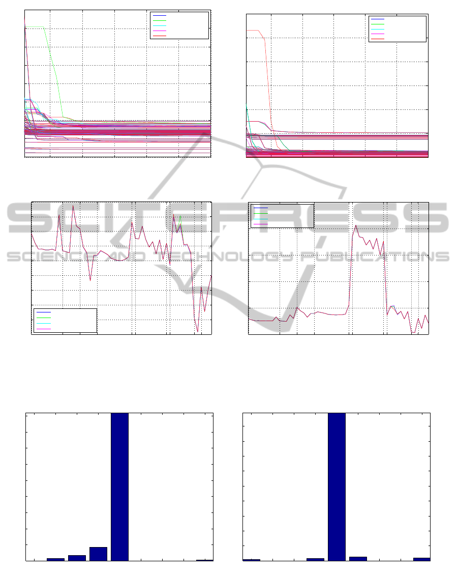
Figure 2: Results using non-normalized (a,c,e) and normalized (b,d,f) data for all datasets. Figures (a) and (b) show the
evolution of the reprojection error over the BA iterations for all datasets. Figures (c) and (d) show the final reprojection error
over all the datasets. Different data sets are denoted by their name. Figures (e) and (f) contain histograms of the relative
difference of the final reprojection error for the new parameterization compared to all other parameterizations.
GlobalCameraParameterizationforBundleAdjustment
559
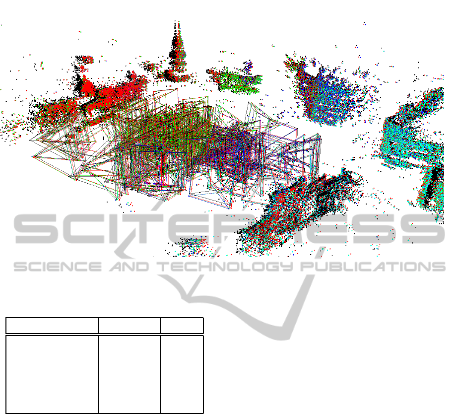
Figure 3: A visualization of a sample from the Trafalgar dataset with 126 cameras after BA using different parameterizations.
The original data is labeled by black color. Results obtained for other parameterizations are colored as in the previous figures.
Table 1: Parameterizations used in experiments.
Parameterization Parameters No. par.
Angleaxis k
11
,a,C 7
4-quaternion k
11
,q,C 8
3-quaternion-tangent k
11
,v,C 7
3-quaternion-local k
11
,q
2
,q
3
,q
4
,C 7
New q,C 7
summary of the parameterizations can be found in ta-
ble 1.
3.1 Results
The results for both normalized and non-normalized
data are shown in Figure 2. We compared the evo-
lution of the reprojection error over each iteration as
well as its final value. One can see in Figures 2(c)
and 2(d) that the new parameterization is converging
to the same value of reprojection error as all the other
parameterizations. The numbers on the x-axis denote
the index of a dataset and the labels separate different
datasets. The same behaviour is observed for all the
parameterizations, with the exception of several out-
liers.
The convergence curves are not always identical
for different parameterizations, Figures 2(a) and 2(b).
We have found that the normalized data are slightly
better suited for BA, as suggested in (Wheeler and
Ikeuchi, 1995), judging from the convergence which
was slightly faster and also more correlated between
different parameterizations.
The histograms in Figures 2(e) and 2(f) show the
relative difference in reprojection error achieved by
our parameterization compared to all other parameter-
izations on all datasets, where by a run we denote a re-
sult of one parameterization on one of the datasets. In
vast majority of cases our parameterization achieved
exactly the same final reprojection error value.
In absence of ground truth data, we compared the
resulting parameters of cameras, i.e. the focal lengths,
camera centers and orientations only among the tested
parameterizations. As in the case of reprojection er-
ror, the resulting parameters after BA were exactly the
same for all parameterizations. The parameters some-
times differed by a similarity transformation and after
registering them, they were the same. Since the quan-
titative results would not be interesting, we show at
least the final reconstruction of one of the datasets us-
ing all parameterizations in Figure 3. Original data is
labeled by black color and the results using different
parameterizations are colored accordingly to previ-
ous figures. The results are almost indistinguishable,
which was also the case for the rest of the datasets.
VISAPP2014-InternationalConferenceonComputerVisionTheoryandApplications
560

4 CONCLUSIONS
In this paper, we proposed a new, global, and non-
redundant (i.e. minimal) parameterization of a per-
spective camera for the Bundle Adjustment. We
discussed the advantages of this parameterization in
comparison to other commonly used parameteriza-
tions. Experiments evaluating the performance in
terms of reducing the reprojection error were con-
ducted on real datasets. The results showed that the
proposed parameterization is achieving the same per-
formance as the other investigated parameterizations
and therefore we conclude that the new parameteriza-
tion is a viable and practical option in BA.
ACKNOWLEDGEMENTS
The work was supported by the EC project FP7-
SME-2011-285839 De-Montes, Technology Agency
of the Czech Republic project TA2011275 ATOM
and Grant Agency of the CTU Prague project
SGS12/191/OHK3/3T/13. Any opinions expressed in
this paper do not necessarily reflect the views of the
European Community. The Community is not liable
for any use that may be made of the information con-
tained herein.
REFERENCES
Agarwal, S., Snavely, N., Seitz, S. M., and R. Szeliski, R.
(2010). Bundle adjustment in the large. In ECCV (2),
pages 29–42.
Barfoot, T., Forbes, J. R., and Furgale, P. T. (2011). Pose
estimation using linearized rotations and quaternion
algebra. Acta Astronautica, 68:101 – 112.
Byr¨od, M. and
˚
Astr¨om, K. (2010). Conjugate gradient bun-
dle adjustment. In Proceedings of the 11th European
conference on Computer vision: Part II, ECCV’10,
pages 114–127, Berlin, Heidelberg. Springer-Verlag.
Craig, J. (2005). Introduction to Robotics: Mechanics and
Control. Addison-Wesley series in electrical and com-
puter engineering: control engineering. Pearson Edu-
cation, Incorporated.
Crandall, D., Owens, A., and Snavely, N. (2011). Discrete-
continuous optimization for large-scale structure from
motion. IEEE Conference on Computer Vision and
Pattern Recognition (2008), 286(26):3001–3008.
Google (2012). Ceres solver.
Hartley, R. I. and Zisserman, A. (2004). Multiple View Ge-
ometry in Computer Vision. Cambridge University
Press, second edition.
Hazewinkel, M. (1987). Encyclopaedia of Mathematics (1).
Encyclopaedia of Mathematics: An Updated and An-
notated Translation of the Soviet ”Mathematical En-
cyclopaedia”. Springer.
Heyden, A. and
˚
Astr¨om, K. (1997). Euclidean reconstruc-
tion from image sequences with varying and unknown
focal length and principal point. pages 438–443.
Heyden, A. and
˚
Astr¨om, K. (1999). Flexible calibration:
minimal cases for auto-calibration. In Computer Vi-
sion, 1999. The Proceedings of the Seventh IEEE In-
ternational Conference on, volume 1, pages 350–355
vol.1.
Jeong, Y., Nister, D., Steedly, D., Szeliski, R., and Kweon,
I.-S. (2010). Pushing the envelope of modern methods
for bundle adjustment. In Proc. IEEE Conf. Computer
Vision and Pattern Recognition (CVPR), pages 1474–
1481.
Konolige, K. (2010). Sparse sparse bundle adjustment.
In British Machine Vision Conference, Aberystwyth,
Wales.
Kuemmerle, R., Grisetti, G., Strasdat, H., Konolige, K., and
Burgard, W. (2011). g2o: A general framework for
graph optimization. In IEEE International Conference
on Robotics and Automation (ICRA).
Lourakis, M. and Argyros, A. (2009). Sba: A software
package for generic sparse bundle adjustment. ACM
Transactions on Mathematical Software, 36:1–30.
Microsoft (2008). Photosynth.
Schmidt, J. and Niemann, H. (2001). Using quaternions
for parametrizing 3-d rotations in unconstrained non-
linear optimization. In VISION, MODELING, AND
VISUALIZATION 2001, pages 399–406. AKA/IOS
Press.
Shum, H., Ke, Q., and Zhang, Z. (1999). Efficient bun-
dle adjustment with virtual key frames: a hierarchi-
cal approach to multi-frame structure from motion.
In Computer Vision and Pattern Recognition, 1999.
IEEE Computer Society Conference on., volume 2,
pages –543 Vol. 2.
Snavely, N. (2011). Bundler: Structure from mo-
tion (sfm) for unordered image collections.
http://phototour.cs.washington.edu/bundler/.
Triggs, B., Mclauchlan, P., Hartley, R., and Fitzgibbon, A.
(2000). Bundle adjustment - a modern synthesis. In
Vision Algorithms: Theory and Practice, LNCS, pages
298–375. Springer Verlag.
Wheeler, M. and Ikeuchi, K. (1995). Iterative estimation of
rotation and translation using the quaternion.
GlobalCameraParameterizationforBundleAdjustment
561
