
Color Supported Generalized-ICP
Michael Korn, Martin Holzkothen and Josef Pauli
Lehrstuhl Intelligente Systeme, Universit
¨
at Duisburg-Essen, 47057 Duisburg, Germany
Keywords:
Iterative Closest Point (ICP), Generalized-ICP (GICP), Point Cloud Registration.
Abstract:
This paper presents a method to support point cloud registration with color information. For this purpose
we integrate L
?
a
?
b
?
color space information into the Generalized Iterative Closest Point (GICP) algorithm, a
state-of-the-art Plane-To-Plane ICP variant. A six-dimensional k-d tree based nearest neighbor search is used
to match corresponding points between the clouds. We demonstrate that the additional effort in general does
not have an immoderate impact on the runtime, since the number of iterations can be reduced. The influence
on the estimated 6 DoF transformations is quantitatively evaluated on six different datasets. It will be shown
that the modified algorithm can improve the results without needing any special parameter adjustment.
1 INTRODUCTION
The Iterative Closest Point (ICP) algorithm has be-
come a dominant method for dealing with range im-
age aligning in the context of 3D Reconstruction, Vi-
sual Odometry and Self Localisation and Mapping
(SLAM). Especially over the last three years, it has
gained in popularity as range cameras have become
low priced and highly available for everyone. How-
ever, since it usually relies only on geometry, this al-
gorithm has its weaknesses in environments with lit-
tle 3D structure or symmetries. Fortunately, many of
the new range cameras are equipped with a color sen-
sor – as a consequence, the logical step is to improve
the ICP algorithm by using texture information. To
preserve the advantages of ICP – simplicity and per-
formance – we are interested in integrating colors di-
rectly into the ICP algorithm. Alternatively, for ex-
ample it is equally conceivable to estimate an initial
alignment in a preprocessing step via Scale Invari-
ant Feature Transform (SIFT) as described in (Joung
et al., 2009). Although such an extension to ICP has
been at the core of several research efforts, there is
still no satisfactory answer as to how ICP should actu-
ally be combined with color information. In (Johnson
and Kang, 1999), the distance function for the near-
est neighbor search of a traditional ICP is extended
by color information. In a similar approach (Men
et al., 2011) use just the hue from the Hue-Saturation-
Lightness (HSL) model to achieve illumination in-
variance. In (Druon et al., 2006), the geometry data is
segmented by associated color in the six color classes
red, yellow, green, cyan, blue and magenta. In ac-
cordance with a valuation method, the most promis-
ing class is then chosen to solve the registration prob-
lem. Nevertheless, the possibilities of said ICP and
color information combination have not been conclu-
sively investigated yet. Especially recent ICP variants
should be considered.
This paper presents a way to integrate color in-
formation represented in L
?
a
?
b
?
color space into
Generalized-ICP (GICP), a state-of-the-art variant of
the ICP algorithm. We focused on the question,
how far this Plane-To-Plane ICP algorithm can benefit
from color information and to what extent the runtime
will be effected.
Section 2 summarizes some required background
knowledge, 3 describes our modifications to GICP, 4
details our experiments and results. In the final sec-
tion we discuss our conclusions and future directions.
2 BACKGROUND
We will introduce essential background knowledge
with regard to GICP and our modifications. In partic-
ular, the characteristics of a Plane-To-Plane ICP will
be considered.
2.1 ICP Algorithm
The Iterative Closest Point (ICP) algorithm was de-
veloped by Besl and McKay (Besl and McKay, 1992)
to accurately register 3D range images. It aligns two
point clouds by iteratively computing the rigid trans-
592
Korn M., Holzkothen M. and Pauli J..
Color Supported Generalized-ICP.
DOI: 10.5220/0004692805920599
In Proceedings of the 9th International Conference on Computer Vision Theory and Applications (VISAPP-2014), pages 592-599
ISBN: 978-989-758-009-3
Copyright
c
2014 SCITEPRESS (Science and Technology Publications, Lda.)
formation between them. Over the last 20 years, many
variants have been introduced, most of which can be
classified as affecting one of six stages of the ICP al-
gorithm (Rusinkiewicz and Levoy, 2001):
• Selection of some set of points in one or both
point clouds.
• Matching these points from one cloud to samples
in the other point cloud.
• Weighting the corresponding pairs appropriately.
• Rejecting certain pairs based on looking at each
pair individually or considering the entire set of
pairs.
• Assigning an error metric based on the point
pairs.
• Solving the optimization problem.
Since all ICP variants might get stuck in a local min-
imum, they are generally only suitable if the distance
between the point clouds is already small enough at
the beginning. This insufficiency is often handled by
estimating an initial transformation with methods or
algorithms that converge to the global minimum but
with lower precision. Following this procedure, an
ICP algorithm is then used to improve the result by
performing a Fine Registration (Salvi et al., 2007). In
other scenarios, no guess of the initial transformation
is needed because the difference between the mea-
surements is sufficiently small. In many applications,
the point clouds are created and processed at such a
high rate (up to 30Hz) that this precondition is met.
The simplest concept based on (Besl and McKay,
1992) with an improvement proposed by (Zhang,
1994) is illustrated in 1 and is often referred to as
Standard ICP (cf. (Segal et al., 2009)). The algo-
rithm requires the model point cloud A and the data
point cloud B in order to estimate the transforma-
tion T between them. Additionally, a rough estimate
transformation T
0
can be considered. If the unknown,
true transformation between the point clouds is small
enough, the initial transformation can be set to the
identity.
In every iteration, each of the N points of the data
point cloud is transformed with the current transfor-
mation estimation and matched with its correspond-
ing point from the model A (line 4). Matches are re-
jected if the Euclidean distance between the pairs ex-
ceeds d
max
, by setting the weight to 0 or 1 accordingly.
After solving the optimization problem in line 11, the
next iteration starts. Usually the algorithm converges
if the difference between the estimated transforma-
tion of two subsequent iterations becomes small or if
a predefined number of iterations is reached.
Algorithm 1: Standard ICP.
Input: Pointclouds: A = {a
1
, . .. , a
M
}, B = {b
1
, . . . , b
N
}
[0] An initial transformation T
0
Output: The transformation T which aligns A and B
1: T ← T
0
2: while not converged do
3: for i ← 1 to N do
4: m
i
← FindClosestPointInA(T b
i
)
5: if km
i
− T b
i
k
2
≤ d
max
then
6: w
i
← 1
7: else
8: w
i
← 0
9: end if
10: end for
11: T ← argmin
T
∑
i
w
i
kT b
i
− m
i
k
2
2
12: end while
2.2 GICP Algorithm
The Standard ICP algorithm is a Point-To-Point ap-
proach, which means that it tries to align all matched
points exactly by minimizing their Euclidean dis-
tance. This doesn’t take into account that an exact
matching is usually not feasible because the different
sampling of the two point clouds leads to pairs with-
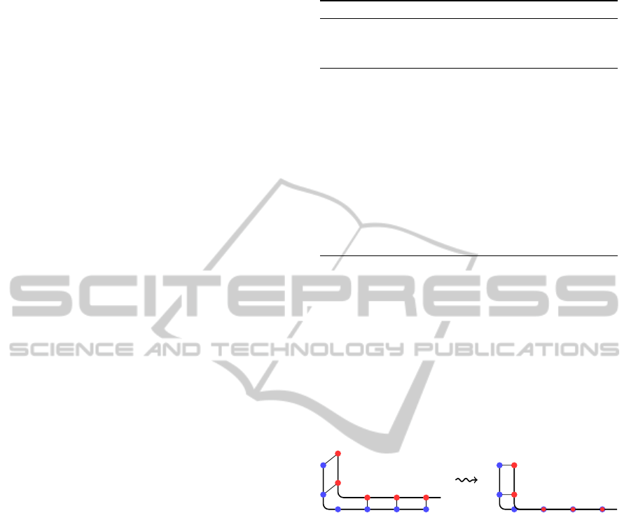
out perfect equivalence. 1 illustrates two point clouds,
both being different samplings of the same scene. The
Figure 1: The exact Point-To-Point matching of the Stan-
dard ICP can lead to a poor alignment of two samplings
(blue and red point clouds) of the same scene.
right part of this figure shows the result when apply-
ing Standard ICP. Three of the correspondences have
a distance close to zero while the other two pairs still
have a significant offset – reducing it could improve
the result. Obviously, the red data cloud should be
shifted to the left for a perfect alignment, but this
would increase three of the pairs’ distances while re-
ducing only two, which would deteriorate the result
in terms of the strict Point-To-Point metric.
To overcome this issue, some variants of ICP take
advantage of the surface normal information. While
Point-To-Plane variants consider just the surface nor-
mals from the model point cloud, Plane-To-Plane
variants use the normals from both model and data
point cloud. The Generalized-ICP (GICP) algorithm
introduced in (Segal et al., 2009) belongs to the sec-
ond category. It uses a probabilistic model to modify
the error function in line 11 of 1 by assigning a co-
variance matrix to each point. This is based on the
ColorSupportedGeneralized-ICP
593

assumption that every measured point results from an
actually existing point and the sampling can be mod-
eled by a multivariate normal distribution. The out-
come of the derivation in (Segal et al., 2009) is the
new error function
T ← argmin
T
∑
i
d
(T)
T
i
C
A
i
+ TC
B
i
T
T
−1
d
(T)
i
(1)
where d
(T)
i
= a
i
− Tb
i
with covariance matrices C
A
i
and C
B
i
(assuming that all points which could not be
matched were already removed from A and B and that
a
i
corresponds with b
i
). This formula resembles the
Mahalanobis distance – only the square root is miss-
ing. An appropriate selection of C
A
i
and C
B
i
can re-
produce the error function of the Standard ICP or a
Point-To-Plane variant (Segal et al., 2009). It is pro-
posed to use the covariance matrix
ε 0 0
0 1 0
0 0 1
for a point with the surface normal e
1
= (1, 0, 0)
T
,
where ε is a small constant representing the covari-
ance along the normal. In general, this covariance
matrix must be rotated for every point depending on
its surface normal. In 2, the covariance matrices are
visualized as confidence ellipses: The position of a
point is known with high confidence along the nor-
mal, but the exact location in the plane is unsure.
Figure 2: The confidence ellipses show how the probabilis-
tic Plane-To-Plane model of the Generalized-ICP works.
We have decided to build on GICP because we
expect to get better results compared with other ICP
variants. Particular worthy of mention is the low
sensitivity to the choice of the distance d
max
(line 5
of 1). In general, if d
max
is selected too small, the
probability of convergence to an entirely wrong local
minimum is high and the number of iterations may
go up. For d
max
→ ∞, the estimated transformation
increasingly loses accuracy, yet GICP still shows a
better robustness in comparison with Standard ICP.
There is a direct connection to the observation that
an ICP algorithm works best if the data point cloud
is a subset of the model point cloud. It may happen
that the data cloud contains points with no adequate
correspondence in the model due to missing points
caused by occlusion or a slight offset of the measured
area. Nevertheless, many ICP variants consider these
points until the distance of the false pairs exceeds
d
max
, whereas in GICP this effect is automatically re-
duced since such points often lie on a plane and the
distance along the surface normal is very small.
2.3 L
?
a
?
b
?
Color Space
The data from color cameras is usually provided in
an RGB color space. Unfortunately, this color model
is not well-suited to determine the difference between
colors because it is not perceptually uniform. This
means that the Euclidean distance between two RGB
colors is not proportional to the perceived difference
of these colors (Paschos, 2001). In 1976, the Interna-
tional Commission on Illumination (CIE) introduced
the L
?
a
?
b
?
color space (or CIELAB), which is a color-
opponent space with dimension L
?
for lightness and
a
?
and b
?
for the color-opponent dimensions. 3 illus-
trates how the a
?
axis corresponds to red-green pro-
portion and the b
?
axis determines yellow-blue pro-
portion. The L
?
a
?
b
?
color space aspires to perceptual
L
?
= 0
L
?
= 100
−a
?
+a
?
−b
?
+b
?
Figure 3: Illustration of the L
?
a
?
b
?
color space.
uniformity and is also appropriate to deal with high il-
lumination variability (Paschos, 2001) (Macedo-Cruz
et al., 2011).
3 INTEGRATING COLOR
The GICP is a promising approach and we decided
to build on it. Because of the significance of the
Euclidean distance, it makes sense to combine the
L
?
a
?
b
?
color space with a geometric based algorithm.
There are several possibilities to integrate color infor-
mation into GICP. According to the list in subsection
VISAPP2014-InternationalConferenceonComputerVisionTheoryandApplications
594

2.1, the steps selection, matching, weighting, rejec-
tion and the error metric could be improved.
We have major doubts to modify the selection step
as in (Druon et al., 2006); the division of both point
clouds into different color classes leads to an extreme
thinning of the clouds and therefore an inadmissible
loss of information. Weighting or rejecting point pairs
based on their colors could depreciate wrong corre-
spondences, but this doesn’t automatically promote
the creation of better correspondences. Maybe this
could increase the dominance of good pairs. In any
case, the number of considered pairs would be re-
duced. This can be problematic, as particularly during
the first iterations of GICP, many correspondences are
wrong, but serviceable for converging to the correct
solution.
An interesting idea is to include the color informa-
tion into the error metric. Unfortunately, this would
go beyond the concept of an ICP algorithm. By re-
ducing the geometric distance of point pairs, it is not
possible to reduce the color distance of the pairs. Con-
sequently, it would no longer be enough to consider
just point pairs.
We have selected the matching step to realize our
modification. This is one of the most crucial steps of
the ICP algorithm regarding the quality of the final
registration. The future stages of the algorithm are
largely dependant on this step, since a high number of
incorrectly associated points obviously cannot lead to
a good registration result.
One of the main advantages of Standard ICP is
its simplicity, which allows to use very efficient data
structures for its matching step, namely k-d-trees
(Bentley, 1975). Since we want to retain this ben-
efit, we chose to simply extent the problem of find-
ing the nearest neighbor from a three-dimensional to
a six-dimensional space, which includes three addi-
tional components for L
?
a
?
b
?
color values. As a con-
sequence, a point has the following structure:
p
i
=
x
i
y
i
z
i
L
i
a
i
b
i
T
Since there is no natural relation between position and
color distance, we introduce a color weight α:
p
α,i
=
x
i
y
i
z
i
α L
i
α a
i
α b
i
T
.
The weight α also serves as scale between geometric
distance of the points and color distance to ensure that
they are in the same order of magnitude. Since the
matching is still based on the Euclidean distance
q
(x
i
− x
j
)
2
+ (y
i
− y
j
)
2
+ (z
i
− z
j
)
2
+
α
2
((L
i
− L
j
)
2
+ (a
i
− a
j
)
2
+ (b
i
− b
j
)
2
)
between points p
α,i
and p
α, j
, the correspondences can
be determined by a nearest neighbor search using a
k-d tree, where α affects the priority of the color dif-
ferences. For α = 0, the resulting transformation ex-
actly equals the output of the original GICP.
The choice of the right weight depends very much
on the sensor hardware. The scale part of α can be
determined relatively easily. To get a first idea of the
scale, the metric (meter or millimeter) of the range
images must be considered and whether the sensor
works in close-up or far range. But a good choice
of the weight also depends on range image and color
image noise.
4 EVALUATION AND RESULTS
We evaluated the color supported Generalized-ICP
with six datasets from (Sturm et al., 2012) and one
self-created point cloud pair. All datasets were ob-
tained from a Microsoft Kinect or an Asus Xtion
camera and d
max
= 0.2 m was used for all examined
scenes. The datasets from (Sturm et al., 2012) include
highly accurate and time-synchronized ground truth
camera poses from a motion capture system, which
works with at least 100Hz and up to 300Hz.
Our implementation uses the Point-Cloud-Library
(PCL) (Rusu and Cousins, 2011). The PCL already
contains a GICP implementation which is strictly
based on (Segal et al., 2009) and also offers the pos-
sibility of modification. We measured the runtimes
on an Intel Core i7-870 with PC1333 DDR3 mem-
ory without any parallelization. The runtimes do not
include the application of the voxel grid filter
1
, but
they consider the transformation of the color space.
To guarantee a fair comparison, we always applied
the unmodified GICP for α = 0. We removed points
from all point clouds with a Z-coordinate greater than
3m, because we observed that the noise of points with
a greater distance generally degrades the results, re-
gardless of the color weight.
For the quantitative assessment, we determined
the transformations between the point clouds of the
different datasets. To avoid incorporating another al-
gorithm for Coarse Registration, the temporal offset
between the aligned point clouds was chosen small
enough to use the identity as the initial transforma-
tion.
In the following evaluation, we will first of all ex-
amine the influence of the color weight. After that,
we will evaluate the benefit of our modifications.
1
A 3D voxel grid is created over a point cloud. All the
points located in the same cell will be approximated with
their centroid and their average color.
ColorSupportedGeneralized-ICP
595

0 1 2 3 4
5 6
7 8 9
·10
−2
0
2
4
6
8
color weight α
iterations runtime in 100ms
translation error in cm
rotation error in
◦
Figure 5: Influence of color weight on number of iterations, runtime, translation error and rotation error. Average values of
1977 aligned point cloud pairs from ’freiburg2 desk’ (a typical office environment with a lot of geometric structure).
Figure 4: Dataset ’freiburg2 desk’ from (Sturm et al., 2012)
containing a typical office scene.
4.1 Evaluating Color Weight
In a typical scene captured with the Kinect, the max-
imum L
?
a
?
b
?
color space distance is approximately
120 and the geometric distance of the furthest points
is about 3.5m. Apart from that, one must consider
that the geometric distance of matched point pairs is
smaller than 0.2 m and the maximum color distance
in a local area is approximately 40. As a conse-
quence, the scale part of the color weight α (which
ensures color and geometric distances are in the same
order of magnitude) should be roughly in the range
of 0.005 to 0.029. 4 was taken from the sequence
’freiburg2 desk’. The Kinect was moved around a
typical office environment with two desks, a computer
monitor, keyboard, phone, chairs, etc. We applied our
color supported GICP to this dataset with different
color weights. The cell size of the voxel grid filter
is 2cm and the frame offset is 1 s (every 30
th
frame).
5 illustrates the influence of α on the number of it-
erations, runtime, translation error and rotation error.
The results represent the average of 1977 registered
point cloud pairs. A minimum of translation and rota-
tion errors is located in the expected range. The color
supported GICP is not too sensitive to a perfect choice
of α since a wide range of α values can be used to im-
prove the results. 0.006 ≤ α ≤ 0.03 seems to be a
good choice. Furthermore, a reduction of the num-
ber of iterations can be observed due to better point
matchings even in early iterations. However, as a con-
sequence of the more complex algorithm, the runtime
becomes worse, but considering the reduced errors it
is still acceptable. A peculiarity is depicted at the be-
ginning of the curves in 5. Although the number of it-
erations is decreasing, the runtime is extending. This
highlights that the convergence of the optimization
process (Broyden-Fletcher-Goldfarb-Shanno method
which approximates Newton’s method) has a large
impact on the runtime. The optimization takes longer
with a well-chosen color weight, since the algorithm
performs greater adjustments of the transformation in
every iteration. Nevertheless, the final transformation
is closer to the reference and the errors are smaller.
It can be noted that even in a scene with sufficient
geometric structure – where one could expect no ap-
preciable advantage of using color information – the
errors can still be reduced.
In contrast to the previous scene with plenty of
geometric information, 7 shows the influence of α
for an environment without any structure (shown in
6). No voxel grid filter has been used and the
frame offset is
1
3
s (every 10
th
frame). In the dataset
’freiburg3 nostructure texture far’, the Asus Xtion is
moved in two meters height along several conference
posters on a planar surface. As expected, the use
of color information leads to a significant improve-
ment of the results. Since the original GICP needs an
unusually large number of iterations to converge, the
color supported GICP even has a lower runtime. This
is because the original GICP often drifts to a wrong
VISAPP2014-InternationalConferenceonComputerVisionTheoryandApplications
596

0 1 2 3 4
5 6
7 8 9
·10
−2
0
10
20
30
40
color weight α
iterations
runtime in s
translation error in cm
rotation error in
◦
Figure 7: Influence of color weight on number of iterations, runtime, translation error and rotation error. Average values of
279 aligned point cloud pairs from ’freiburg3 nostructure texture far’ (planar surface with posters).
Figure 6: Dataset ’freiburg3 nostructure texture far’ (left)
and ’freiburg3 nostructure texture near withloop’ (right).
direction, which is also indicated by the huge trans-
lation errors. Surely, this can be a peculiarity of the
dataset and should not be generalized. The drift can
be explained with range image noise. The application
of a voxel grid filter can significantly reduce this drift
and therefore the number of iterations and resulted er-
rors decrease.
Overall, the curves decrease very early and stag-
nate at a lower level, because a small color weight
is already sufficient to the color information becomes
dominant over the range image noise. In the absence
of geometric features, the sensitivity to the choice of
the color weight is less than in the previously dis-
cussed dataset. As the color information becomes
more important, the color weight should be higher.
With respect to all examined datasets, a good choice
is α = 0.024 ± 0.006.
4.2 Benefit of Color Support
In addition to the two scenes of the previous subsec-
tion, the suitability of color support will be shown for
other scenes and for different cell sizes of the voxel
grid filter. In order to preserve a better overview, the
color weight will be set to a fixed value of α = 0.024
Figure 8: Dataset ’freiburg1 room’ containing a typical of-
fice room with much motion blur due to fast movement.
for all experiments in this subsection. The results are
summarized in 1 and will be explained and discussed
in the remainder of this section. The first dataset was
already discussed above. Both the original GICP and
the color supported GICP benefit from the voxel grid
filter. It is noticeable, though, that the effect on the
modified GICP is smaller, which can be explained by
the negative influence of smoothing the color infor-
mation.
The next dataset was chosen to indicate the effects
of fast camera movements, particularly as this often
causes more problems for the color images as for the
range images. This dataset was produced in a typical
office room and is shown in 8. The camera was moved
at high speed on a trajectory through the whole office.
Therefore, a major part of the color images contains
a lot of motion blur. Nevertheless, using color infor-
mation improves the results, however, sharp images
would probably have a stronger effect.
In the next two sequences (depicted in 6), the cam-
era was moved along a textured, planar surface. In
one case, which was already considered in the previ-
ous subsection, the height was two meters and in the
other case it was one meter. In this scene the voxel
grid filter has a particularly significant impact on the
ColorSupportedGeneralized-ICP
597

Table 1: Comparison of the original GICP and the color supported GICP with α = 0.024 based on average values of number
of iterations, runtime, translation error and rotation error. Six datasets (names were shortened) from (Sturm et al., 2012) and
one self-created point cloud pair are considered under different cell sizes of the voxel grid filter (’-’ means no voxel grid filter
was used).
dataset voxel grid iterations runtime (ms) error (cm /
◦
)
(pairs, time offset) cell size (cm) GICP color GICP GICP color GICP GICP color GICP
freiburg2 desk - 17.05 11.85 15544 22501 8.590 / 2.984 4.105 / 1.707
(1977, 1s) 2 7.90 5.79 322 444 4.093 / 1.244 2.290 / 0.907
3 7.13 5.52 136 176 3.876 / 1.167 2.520 / 0.992
freiburg1 room - 17.54 14.50 40797 72732 14.987 / 5.543 11.047 / 4.443
(1323, 1/3s) 2 11.54 9.56 479 770 14.963 / 4.559 10.801 / 3.225
3 10.85 8.92 176 256 15.079 / 4.348 10.713 / 3.238
f3 nostructure texture far - 38.57 15.86 18199 14689 20.710 / 2.250 4.061 / 1.003
(279, 1/3s) 2 4.87 5.32 262 411 10.313 / 0.966 7.507 / 0.939
3 3.84 3.87 114 152 10.224 / 0.958 8.331 / 0.980
f3 nostructure texture near - 6.14 10.27 5140 15101 12.755 / 3.485 8.727 / 2.440
(1565, 1/2s) 2 2.88 3.49 89 130 12.405 / 3.497 10.859 / 3.326
3 2.71 3.12 39 53 12.356 / 3.506 11.102 / 3.402
f3 structure texture far - 9.43 6.85 7463 9864 2.640 / 0.563 1.776 / 0.522
(837, 1s) 2 5.15 4.29 304 386 2.334 / 0.459 1.635 / 0.445
3 4.64 3.88 132 159 2.388 / 0.460 1.987 / 0.452
f3 structure texture near - 10.036 9.02 22442 28145 4.793 / 1.040 4.003 / 0.988
(974, 1s) 2 6.44 6.10 175 275 5.548 / 1.261 5.248 / 1.104
3 5.76 5.64 70 102 5.679 / 1.222 5.573 / 1.195
office corridor - 8 10 9057 20987 18.705 / 0.976 1.691 / 1.850
(1, 21.6cm / 4
◦
) 2 8 7 565 865 16.959 / 0.764 1.854 / 0.336
3 7 8 220 325 17.109 / 1.383 1.241 / 0.564
Figure 9: Dataset ’freiburg3 structure texture far’ (left) and
’freiburg3 structure texture near’ (right).
number of iterations and the runtime. Lower range
image noise and less points lead to sooner conver-
gence and – in case of two meters height – a shorter
drift. Apart from suppressing the drift, the voxel grid
filter has no impact on the original GICP since (inde-
pendently of the smoothing) there is no useful struc-
ture information. A greater cell size of the voxel grid
filter degrades the result of the color GICP since it
removes too much valuable information.
Because of reducing the errors on ’freiburg2 desk’
with color information, the evaluation also includes
the next two datasets shown in 9. The color-supported
GICP can only slightly improve the results because
the scene contains an unusually distinctive 3D struc-
ture that occurs very rarely in real applications.
Finally, a self-created point cloud pair has been
captured in an office corridor, representing a more
Figure 10: The first row shows two point clouds of an office
corridor. The lower row depicts their alignment with the
original GICP (left) and with color support (right).
common case, in which the original GICP fails to
reach a good alignment (see 10). This scene conveys
only enough structural information to restrict three of
the total six degrees of freedom. The alignment could
still be rotated and translated like two ordinary planes
without significantly affecting the error in terms of the
plane-to-plane metric. The integration of colors, how-
ever, leads to a remarkable improvement.
Overall, the color supported GICP achieves a re-
VISAPP2014-InternationalConferenceonComputerVisionTheoryandApplications
598

duction of the average error. The concrete benefit de-
pends on the scene, but considering only the accuracy
of the estimated transformation there are no disadvan-
tages. In most cases, the runtime rises, but this is
moderated due to the reduction of the number of it-
erations.
5 CONCLUSIONS
In this paper, we present a method to integrate color
information directly into the GICP algorithm. Due
to the type of modification, only one new parameter
has to be set and it was possible to give a general
recommendation that shows good results in various
scenes. It has been demonstrated that the estimated
transformations are generally more accurate and the
number of iterations is reduced, even though the run-
time rises. Color support was shown to be particularly
worthwhile in environments with texture and less 3D
structure. Consequently, switching between the orig-
inal and the modified GICP depending on the pres-
ence of structure features is reasonable. A negative
impact on the resulting transformations could not be
observed during the experiments, not even if the color
images had a poor quality due to motion blur.
Compared to (Johnson and Kang, 1999) and (Men
et al., 2011), the GICP benefits less from color in-
tegration than the Standard ICP algorithm. This can
be explained in part by comparing GICP with Stan-
dard ICP: The measured translation and rotation er-
rors of the Standard ICP on all examined structured
scenes are approximately twice as high as those of
GICP. And since GICP already performs much better,
the benefit of any modification will be less in abso-
lute terms. In addition, GICP reduces the distances
of corresponding points in the direction of the sur-
face normals. While the information obtained from
the 3D structure is useful to correct the point align-
ments along the surface normals, the color informa-
tion is helpful to align the points along the surfaces.
For future work, we plan to extend the error met-
ric and thus also the concept of the GICP to allow
structure features and color features to act in different
directions.
REFERENCES
Bentley, J. L. (1975). Multidimensional binary search trees
used for associative searching. Communications of the
ACM, 18(9):509–517.
Besl, P. J. and McKay, N. D. (1992). A method for regis-
tration of 3-d shapes. IEEE Transactions on Pattern
Analysis and Machine Intelligence, 14(2):239–256.
Druon, S., Aldon, M. J., and Crosnier, A. (2006). Color
constrained icp for registration of large unstructured
3d color data sets. In Proc. of the IEEE International
Conference on Information Acquisition, pages 249–
255.
Johnson, A. E. and Kang, S. B. (1999). Registration and in-
tegration of textured 3d data. Image and Vision Com-
puting, 17:135–147.
Joung, J., An, K. H., Kang, J. W., Chung, M.-J., and Yu, W.
(2009). 3d environment reconstruction using modified
color icp algorithm by fusion of a camera and a 3d
laser range finder. In Intelligent Robots and Systems,
pages 3082–3088.
Macedo-Cruz, A., Pajares, G., Santos, M., and Villegas-
Romero, I. (2011). Digital image sensor-based assess-
ment of the status of oat (avena sativa l.) crops after
frost damage. Sensors, 11(6):6015–6036.
Men, H., Gebre, B., and Pochiraju, K. (2011). Color point
cloud registration with 4d icp algorithm. In Proc. of
the IEEE International Conference on Robotics and
Automation, pages 1511–1516.
Paschos, G. (2001). Perceptually uniform color spaces for
color texture analysis: An empirical evaluation. IEEE
Transactions on Image Processing, 10(6):932–937.
Rusinkiewicz, S. and Levoy, M. (2001). Efficient variants
of the icp algorithm. In Proc. of the 3rd International
Conference on 3-D Digital Imaging and Modeling,
pages 145–152.
Rusu, R. B. and Cousins, S. (2011). 3d is here: Point cloud
library (pcl). In International Conference on Robotics
and Automation, Shanghai, China.
Salvi, J., Matabosch, C., Fofi, D., and Forest, J. (2007).
A review of recent range image registration methods
with accuracy evaluation. Image and Vision Comput-
ing, 25:578 – 596.
Segal, A., Haehnel, D., and Thrun, S. (2009). Generalized-
icp. Robotics: Science and Systems V.
Sturm, J., Engelhard, N., Endres, F., Burgard, W., and Cre-
mers, D. (2012). A benchmark for the evaluation of
rgb-d slam systems. In Proc. of the International Con-
ference on Intelligent Robot Systems (IROS).
Zhang, Z. (1994). Iterative point matching for registration
of free-form curves and surfaces. International Jour-
nal of Computer Vision, 13(2):119–152.
ColorSupportedGeneralized-ICP
599
