A Constraint Programming Approach for Managing End-to-end

Requirements in Sensor Network Macroprogramming

Farshid Hassani Bijarbooneh

, Animesh Pathak

, Justin Pearson

Valerie Issarny

and Bengt Jonsson

Uppsala University, Department of Information Technology, Box 337, SE-75105, Uppsala, Sweden

INRIA Paris, Rocquencourt, France

Keywords:

Sensor Networks, Macroprogramming, Constraint Programming, Non-functional Requirements, Task Map-

ping.

Abstract:

Though several high-level application development (macroprogramming) approaches have been proposed in

literature for wireless sensor networks (WSN), there is a need to enable support for expressing and support-

ing end-to-end non-functional constraints such as latency in WSN macroprograms. We augment an existing

macroprogramming language and its compilation process to enable the speciﬁcation of end-to-end require-

ments, and propose task mapping algorithms to satisfy those requirements through a constraint programming

approach. Through evaluations on realistic application task graphs, we show that our constraint programming

model can effectively capture the end-to-end requirements and efﬁciently solves the combinatorial problem

introduced.

1 INTRODUCTION

Sensor network macroprogramming refers to the de-

velopment of Wireless Sensor Network (WSN) appli-

cations at the system level (as opposed to at the node

level), and holds the promise of enabling not just sys-

tems programmers (as is the case today) but also do-

main experts (e.g., architects, biologists, city planners

etc.) to develop WSN applications. A sizeable body

of work exists in this area (Mottola and Picco, 2011),

with programming styles ranging from Haskell-like

functional languages (Newton et al., 2007) to Python-

like imperative ones (Gummadi et al., 2005).

To complement the above, algorithms have been

developed to convert the high level descriptions to

node-level code by solving problems such as optimal

task-mapping in order to satisfy non-functional prop-

erties. While existing approaches focus on system-

wide or node-level goals, such as minimising total

energy consumption or minimising the maximum en-

ergy consumed by any node, work on managing end-

to-end requirements (e.g., minimising the latency be-

tween the sensing of a phenomenon and the resulting

action) in WSN macroprogramming is largely miss-

ing.

The focus of this paper is precisely the above kind

of scenarios, where the developer is interested in min-

imising an end-to-end property while mapping tasks

on the nodes in a particular sensor network deploy-

ment. A classic case would be a highway trafﬁc man-

agement application (e.g., the one used in (Mottola

et al., 2007)), where local regulations might need a

particular deployment to provide guarantees between,

say, the sensing of a trafﬁc jam (speed = 0) and the

actuation of the ramp signals to red in order to stop

more cars from coming in. Similar latency restrictions

apply in the case of, for example, trafﬁc lights con-

trolling access to a railroad crossing (US Department

of Transportation, Federal Highway Administration,

2012).

We base our work on the Abstract Task Graph

(ATaG) macroprogramming language (Bakshi et al.,

2005b), based on the data-driven macroprogramming

paradigm, where the developer breaks up the func-

tionality of their application into tasks that interact

with each other only using the data items that they

produce and consume, and do not share any state oth-

erwise. This technique is shown to be especially use-

ful in specifying a wide range of sense-and-respond

applications (Pathak et al., 2007). ATaG includes an

extensible, high-level programming model to specify

the application behaviour, and a corresponding node-

level run-time support, the data-driven ATaG runtime

(DART) (Bakshi et al., 2005a). The compilation of

Hassani Bijarbooneh F., Pathak A., Pearson J., Issarny V. and Jonsson B..

A Constraint Programming Approach for Managing End-to-end Requirements in Sensor Network Macroprogramming.

DOI: 10.5220/0004715200280040

In Proceedings of the 3rd International Conference on Sensor Networks (SENSORNETS-2014), pages 28-40

ISBN: 978-989-758-001-7

 2014 SCITEPRESS (Science and Technology Publications, Lda.)

ATaG programs consists of mapping the high-level

ATaG abstractions to the functionality provided by

DART, thus involving a task-mapping process. While

the ATaG compiler currently supports task-mapping

while optimising node-level energy properties, it does

not have support for end-to-end properties such as la-

tency.

The main related work to ours is (Pathak and

Prasanna, 2010), where the authors optimised task-

mapping for energy-related metrics using an MIP,

and (Hassani Bijarbooneh et al., 2011), which used

constraint programming (CP) (Rossi et al., 2006)

to solve this. In (Tian et al., 2005), the authors

only investigate single-hop homogeneous WSNs. We

consider multi-hop heterogeneous networks including

routing costs. To the best of our knowledge, there has

been no work addressing a CP approach for a general

case of task mapping in a multi-hop WSN achieving

end-to-end latency optimisation under routing costs.

Works such as the one by Wu et. al., in (Wu et al.,

2010) are complementary to this, since they perform

runtime evaluation of the WSN, while we focus on

providing feedback to the developer before deploy-

ment. Note that the task mapping problem with end-

to-end requirements is different from those encoun-

tered in traditional distributed systems such as clus-

ters, since in our work, there is a strong relationship

between the physical regions and the sensor nodes, as

well as the constraints enforced by the end-to-end re-

quirements between the tasks and the sensor nodes.

The main contributions of this paper are i) The

formulation of the task-mapping problem arising

out of the need to satisfy end-to-end constraints in

WSN macroprogramming; ii) Constraint program-

ming techniques to solve the latency problem; and

iii) Extension of the approach to address situations

where replication of tasks is allowed to improve la-

tency performance.

We provide background on the macroprogram-

ming language used in Section 2, followed by the

problem deﬁnition in Section 3 and the mathemati-

cal formulation of the optimisation goal in Section 4.

Section 5 presents our CP-based approach, and Sec-

tion 6 discusses the results of our evaluation on a re-

alistic trafﬁc-management application. Section 7 con-

cludes.

2 BACKGROUND

For completeness, in this section we provide some

background on the programming model and compi-

lation process of ATaG programs, as well as the mod-

iﬁcations we have made to the language. For more

TemperatureSampler

AverageTemperature

Calculator

Temperature

every(attachedSensors,

TempSensor)

periodic: 10

oncein(Floor)

anydata

(1,Floor)

Figure 1: ATaG program for data-gathering.

complete details of ATaG, we refer the readers to the

work in (Pathak and Prasanna, 2011).

2.1 Programming Model

ATaG provides a data driven programming model

and a mixed imperative-declarative program speciﬁ-

cation. Developers use a data driven model for spec-

ifying reactive behaviours, and declarative speciﬁca-

tions to express the placement of processing locations

and the patterns of interactions.

The overall structure of computation in an ATaG

program is expressed as a task graph (see Figure 1 for

an example), which consists of the following:

• Abstract Data Items: These represent the in-

formation in the various stages of its processing

through the deployed application.

• Abstract Tasks: These are software entities that

consume and produce instances of abstract data

items. To specify their location and invocation

patterns, they are annotated with instantiation

rules and ﬁring rules respectively.

• Abstract Channels: Abstract tasks and data

items are connected through abstract chan-

nels, which are further annotated with logical

scopes (Mottola et al., 2007), expressing the inter-

est of tasks in only certain instances of data items.

In addition to the above, the developer speci-

ﬁes the internal functionality of each abstract task

in an ATaG program using an imperative lan-

guage such as Java. To interact with the under-

lying runtime system, each task must implement a

handleDataItemReceived() method for each

type of data item that it is supposed to process. The

task can output its data by calling the putData()

method implemented by the underlying runtime sys-

tem.

Figure 1 illustrates an example ATaG program

specifying a data gathering application (Choi et al.,

2004) for building environment monitoring. Sen-

sors within a cluster take periodic temperature read-

AConstraintProgrammingApproachforManagingEnd-to-endRequirementsinSensorNetworkMacroprogramming

ings, which are then collected by the correspond-

ing cluster-head. The TemperatureSampler task rep-

resents the sensing in this application, while the

AverageTemperatureCalculator task takes care of

the collection and computing the average. The

tasks communicate through the Temperature data

item. The TemperatureSampler is triggered ev-

ery 10 seconds according to the periodic ﬁring

rule. The any-data rule requires AverageTemper-

atureCalculator to run when a data item is ready

to be consumed on any of its incoming channels.

The every(<property>,<value>) instantia-

tion rule requires the task to be instantiated on

each node where the particular property has that

value. E.g., the TemperatureSampler task in the ex-

ample will be instantiated on every node equipped

with a temperature device. Since the programmer

requires a single AverageTemperatureCalculator to

be instantiated on every ﬂoor in the building, the

oncein(Floor) instantiation rule is used for this

task. Its semantics is to derive a system partition-

ing based on the values of the node attribute provided

(Floor).

The (1,Floor) annotation on the channel spec-

iﬁes a number of hops counted in terms of how many

system partitions can be crossed, independent of the

physical connectivity. Since Temperature data items

are to be used within one partition (ﬂoor) from where

they generated, they will be delivered to AverageTem-

peratureCalculator instances running on the same

ﬂoor as the task that produced them, as well as ad-

jacent ﬂoors.

2.2 Compilation Process

In the previous section, we described the ATaG data-

driven macroprogramming paradigm. In this section,

we provide a formal deﬁnition of the process of com-

piling data-driven macroprograms to node-level code

using the application given in Figure 1 as an example.

TS ATC

Floor 3

Floor 2

Floor 1

Channel

Composition

Task

Instantiation

Figure 2: An example illustrating the compilation process

of our sample program. Task names have been abbreviated.

2.2.1 Input

The input to the compilation process consists of the

following three components.

Abstract Task Graph (Declarative Part): Formally,

an abstract task graph A(AT, AD, AC) consists of a

set AT of abstract tasks and a set AD of abstract data

items. The set of abstract channels AC can be divided

into two subsets – the set of output channels AOC ⊆

AT × AD and a set of input channels AIC ⊆ AD × AT .

Imperative Code for Each Task: As mentioned ear-

lier, each abstract task is accompanied by code that

details the actions taken when data is received by in-

stances of that task.

Network Description: For every node n in the

target network N, the compiler is also given the

list of sensors and actuators attached to the sensor

node n, as well as, a set of (RegionLabel, RegionID)

attribute-value pairs to denote the membership of the

sensor node n in the regions of the network (e.g.,

{(Floor, 5), (Room, 2)}).

Runtime Library Files: These ﬁles contain the code

for the basic modules of the runtime system that are

not changed during compilation, including routing

protocols etc.

2.2.2 Output

The compilation process generates a distributed appli-

cation for the target network description commiserate

with what the developer speciﬁed in the ATaG pro-

gram. The output consists of the following parts:

Task Assignments: This is a mapping between the

instances of the members of AT onto the nodes in N,

in accordance with their instantiation rules.

The compiler must decide on the mapping to al-

locate the instantiated copies of the abstract tasks in

AT to the nodes in N so as to satisfy all placement

constraints speciﬁed by the developer.

Customised Runtime Modules: The compiler must

customise the DataPool of each node to contain a list

of the data items produced or consumed by the tasks

hosted by it. It also needs to conﬁgure the ATaGMan-

ager module with a list of composed channel annota-

tions, so when a data item is produced, the runtime

can compute the constraints imposed on the nodes

which are hosting the recipient tasks for it.

Cost Estimates: The compiler also reports on the

non-functional aspects of the ﬁnal deployed applica-

tion, informing the developer of the cost of executing

application A on a network N. Note that the actual na-

ture of the cost estimates returned can vary depending

on the developer’s needs. This is the place where this

paper builds upon the existing work, by bringing end-

to-end cost estimates also in the compiler’s purview.

SENSORNETS2014-InternationalConferenceonSensorNetworks

2.2.3 Process Overview

The overall process takes place in the following steps:

Composition of Abstract Channels: In this step,

each path AT

→ AD

→ AT

in the abstract task graph

is converted to an edge AT

→ AT

, resulting in a graph

with only task-task edges, keeping the annotation of

the channel AD

→ AT

Instantiating Abstract Tasks: The instantiated task

graph (ITaG) consists of instances of the tasks de-

ﬁned in AT, connected to each other according to the

channel annotations in A. e.g., due to the (1,Floor)

channel annotation, instances of TemperatureSampler

for ﬂoor i are connected only to instances of Aver-

ageTemperatureCalculator destined for ﬂoors i − 1, i,

and i + 1.

Formally, the ITaG I(T, IC) is a graph whose ver-

tices are in a set T of instantiated tasks and whose

edges are from the set IC of instantiated channels. For

each task AT

in the abstract task graph from which I is

instantiated, there are f (AT

, N) elements in T , where

f maps the abstract task to the number of times it is in-

stantiated in N. IC ⊆ T × T connects the instantiated

version of the tasks. The ITaG I can also be repre-

sented as a graph G(V, A), where V = T and A = IC.

Additionally, each T

in the ITaG has a label indicat-

ing the subset of nodes in N it is to be deployed on.

This overlay of communicating tasks over the target

deployment enables the use of modiﬁed versions of

classical techniques meant for analysing task graphs.

For example, for the application in Figure 2,

since there are seven nodes with attached tem-

perature sensors, f (AT

, N) = 7, following the

every(AttachedSensors,TemperatureSensor

instantiation rule of the TemperatureSampler task.

Similarly, f (AT

, N) = 3, since the AverageTem-

peratureCalculator task is to be instantiated once

on each of the three ﬂoors. The ﬁgure shows one

allocation of the tasks in T , with arrows representing

the instantiated channels in IC (it shows channels

leading to only one instance of AT

for clarity).

Note that the although the ITaG notation captures

the information stored in the abstract task graph

(including the instantiation rules of the tasks and

the scopes of the connecting channels) it does not

capture the ﬁring rules associated with each task. The

compiler’s task involves incorporating the ﬁring rule

information while making decisions about allocating

the tasks on the nodes.

Task Mapping: This task graph with composed

channels is then instantiated on the given target net-

work. Figure 2 illustrates an example of a target net-

work. The nodes are on three different ﬂoors, and

those marked with a thermometer have temperature

sensors attached to them. In this stage, the compiler

computes the mapping M : T → N, while satisfying

the placement constraints on the tasks.

Customisation of Runtime Modules: Based on the

ﬁnal mapping of tasks to nodes, and the composed

channels, the Datapool and ATaGManager modules

are conﬁgured for each node to handle the tasks and

data items associated with it.

2.3 Changes to ATaG

For our work, we augment the above in two ways:

1. The abstract task graph now includes end-to-end

non functional requirements. We use latency in

this paper as an example, but our approach is ap-

plicable to other requirements as well.

2. The network description contains probability esti-

mates of the time it takes for messages to be routes

between nodes in same and neighbouring regions.

Using the above, we can reason about applications

such as the Highway Trafﬁc management application

from (Mottola et al., 2007) (shown in Figure 3), and

answer questions such as “Is it possible to deploy this

application in a given city so that whenever the av-

erage speed of a highway sector goes to 0, the ramp

signal for that sector turns red within 1 second with

98% probability?”. The details of the above are dis-

cussed next.

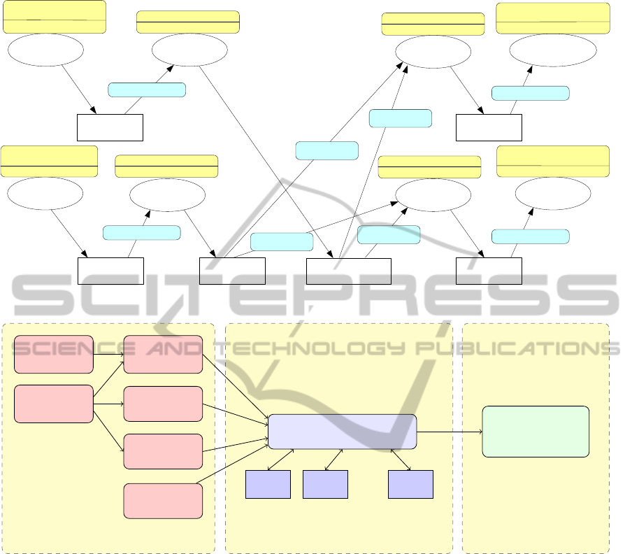
3 PROBLEM DEFINITION

The task mapping problem with end-to-end require-

ments is solved in several steps. In Figure 4 we show

a high-level description of each component involved

in the process of mapping the tasks to the nodes, and

the input and output of our constraint programming

(CP) approach. As explained in programming model

Section 2.1, the developer speciﬁes an abstract task

graph and the rules required to instantiate the tasks.

We preprocess the abstract task graph and instan-

tiate tasks according to the rules speciﬁed in the task

graph, which results in instantiated task graph and

placement constraints, as shown in Figure 4, where

the placement constraints enforce a task to be mapped

only to a subset of sensor nodes.

The probability model, provided by the developer,

speciﬁes the delay distribution for sending a message

between nodes in different and the same regions, as

well as rules on how to combine probability distribu-

tions when messages travel more than one hop. This

allows both independent and dependent message de-

lays to be modelled. In our experiments, for simplic-

AConstraintProgrammingApproachforManagingEnd-to-endRequirementsinSensorNetworkMacroprogramming

AvgQueueLength

RampSignal

Calculator

RampSignal

Displayer

[every(attachedActuators,

rampSignalActuator)]

[anydata]

AvgSpeed

SpeedLimit

Calculator

SpeedLimit

Displayer

[every(attachedActuators,

speedLimitActuator)]

[anydata]

(1, HighwaySector)

RampSampler

VehiclePresence

AvgQueueLength

Calculator

SpeedSampler

RawSpeed

AvgSpeed

Calculator

[every(attachedSensors,

presenceSensor)]

[periodic:10]

[every(attachedSensors,

speedSennsor)]

[periodic:10]

(0,HighwaySector)

[oncein(HighwaySector)]

[anydata]

(1, HighwaySector)

(0,HighwaySector)

(1, HighwaySector)

[oncein(HighwaySector)]

[anydata]

[oncein(HighwaySector)]

[anydata]

[oncein(HighwaySector)]

[anydata]

Figure 3: ATaG Program for the trafﬁc app in (Mottola et al., 2007).

CSP

main

CSP

sub

on path 1

CSP

sub

on path 2

CSP

sub

on path p

·· ·

Network

Description

Abstract

Task Graph

Instantiated

Task Graph

Placement

Constraints

Path Delay

Constraints

Probability

Model

Input

Constraint Programming Model

An Optimal

Mapping of

Tasks to Nodes

Output

Figure 4: Block diagram representing the main components of the task mapping problem with end-to-end requirements.

ity, we have assumed that all distributions are inde-

pendent and normally distributed. In the mathemati-

cal formulation in Section 4, we formulate the aggre-

gation of the delay requirements over the channels.

In our approach, we use a constraint program-

ming model called CSP

main

to perform the compila-

tion process (see Section 2.2). The constraint pro-

gramming model CSP

main

takes the input (instantiated

task graph, placement constraints, and the probability

model), and outputs the optimal mapping from tasks

to nodes. The end-to-end requirements are expressed

in terms of maximum allowed delay between two task

types. For example, we require that the delay for

sending one unit of data between the operational tasks

and the actuating tasks be within a certain threshold.

We ﬁrst convert the end-to-end requirements into a

set of paths (namely path delay constraints), where

each path includes all the tasks (subset of the instanti-

ated tasks) between the two end-points. The probabil-

ity model should specify how the probability distribu-

tion of the delay is computed along each path, given

a mapping from task to nodes, also it should specify

how the probability distribution of delay is computed

if we replicate the tasks along each path.

In our CSP

main

model, we create one CSP

sub

model per path delay constraint, where the CSP

sub

model solves and returns all the valid solutions (map-

ping of tasks to nodes) for one path delay constraint.

The rules provided in the probability model are used

in the CSP

sub

model to check (in polynomial time)

whether a mapping from the tasks to the nodes along

one path is valid. If the requirements on a path can-

not be satisﬁed, then we allow the CSP

sub

model to

replicate the operational tasks on the path to improve

SENSORNETS2014-InternationalConferenceonSensorNetworks

the probability of receiving the data at the end-point.

The valid solutions returned by CSP

sub

for each path

delay constraints are then composed in the CSP

main

model to ﬁnd an optimal mapping of the tasks to the

nodes, minimising the number of replicated tasks. In

the next section, we show how CSP

main

and CSP

sub

are modelled, the probability is computed as we repli-

cate tasks, and how the overall problem is solved to

optimality.

4 MATHEMATICAL

FORMULATION

We ﬁrst instantiate the abstract task on the target net-

work, this process creates several copies of tasks per

region. We then have the following constants in our

model:

• Let N be the set of WSN nodes.

• Let T be the set of instantiated tasks.

• Let A be the set of arcs/edges in the directed

acyclic task graph G = (T, A), with edge (t

, t

) in-

dicating that instantiated task t

is sending data to

task t

• Let D[t

, t

] be the random variable representing

the delay for sending one unit of data from the

task t

to t

, where (t

, t

) ∈ A (the tasks are on the

same edge of the task graph G).

• Let F

, t

] be the cumulative distribution func-

tion (c.d.f) of the random variable D[t

, t

• Let S ⊆ T be the set of (start) tasks where a trig-

gering event is produced.

• Let E ⊆ T be the set of (end) tasks where pro-

ducing an output within a given latency time is

required.

For each task t let node[t] be the decision variable

denoting the node that task t is mapped to, with t ∈ T

and node[t] ∈ N.

As explained in Section 3, the task mapping prob-

lem with end-to-end requirements consists of place-

ment and path delay constraints. The placement con-

straints enforce that a task may be restricted to a suit-

able subset of the sensor nodes, and therefore it can-

not be mapped to any other node. Such placement

constraints are modelled as follows:

node[t] 6= n for every task t that

cannot be mapped to node n

(1)

The path delay constraints ensure that for every path

in the task graph G starting from the tasks in S and

L[t

, t

]L[t

, t

]

D[1, 2] ∼ N(0.5, 1) D[2, 3] ∼ N(0.5, 1)

Figure 5: A path from the task t

to t

via task t

in the task

graph, and the delay random variable D[1, 2] and D[2, 3] for

the edges.

ending with the tasks in E the delay requirements are

satisﬁed:

∀ t

∈ S, t

∈ E,

P(L[t

, t

] ≤ maxDelay) ≥ minProbability

(2)

where L[t

, t

] is a random variable representing the

latency for producing an output data by the task

∈ S in response to a triggering event produced

by the task t

∈ E, and the constants maxDelay

and minProbability are the requirements of the task

graph expressed by the developer. The allowed

maximum delay is represented with maxDelay, and

minProbability is the minimum probability threshold

for the delay requirement probability to hold, where

delay is at most maxDelay. The path delay con-

straints (2) are equivalent to:

∀ t

∈ S, t

∈ E,

, t

](maxDelay) ≥ minProbability

(3)

where F

, t

] is the cumulative distribution function

(c.d.f) of the latency random variable L[t

, t

]. In our

formulation, we consider F

, t

] as an auxiliary vari-

able, that should specify the c.d.f of the delay in the

mapping of the tasks to the nodes on the path from

to t

, and depends on F

[u, v] for each edge (u, v)

in the path from t

to t

, and the rules speciﬁed by the

probability model on how to combine the distributions

over a path.

Typically, the tasks in the set S are operational

tasks, e.g. AverageSpeedCalculator, and the tasks in

the set E are the end-points of the data ﬂow in the

task graph, e.g. RampSignalDisplayer. For exam-

ple, Figure 5 shows a path from the task t

∈ S of

the type AverageSpeedCalculator to the task t

∈ E

of the type RampSignalDisplayer, with the delay ran-

dom variables D[1, 2] and D[2, 3] for the two edges on

the path. In this example, as we consider the delay

random variables D[1, 2] and D[2, 3] independent, it is

trivial to see that the latency L[t

, t

] is equal to the

sum of the delay random variables on each edge:

L[t

, t

] = D[1, 2] + D[2, 3] (4)

We observe that according to the path delay con-

straints (2) the probability P(L[t

, t

] ≤ 3.0) ≥ 0.98

states that for every event triggered by the Average-

SpeedCalculator task t

, we require that in 98% of

AConstraintProgrammingApproachforManagingEnd-to-endRequirementsinSensorNetworkMacroprogramming

···

L[t

, t

]

L[t

, t

]

D[t

, t

]

Figure 6: Path from the task t

to t

via task t

in the task

graph, and the delay random variable D[t

, t

] for sending a

unit of data from task t

to t

the time the RampSignalDisplayer task t

responds

within 3.0 seconds (this corresponds to the require-

ment that in the event of a trafﬁc jam, no more cars

should be allowed onto the highway). If we assume

the delay random variables D[1, 2] and D[2, 3] are

normally distributed with mean 0.5 and variance 1

(N(0.5, 1)), then the c.d.f of L[t

, t

] is also a nor-

mal distribution with mean 1 and variance 2 (sum of

the means and variances). Therefore, the probabil-

ity P(L[t

, t

] ≤ 3.0) ≥ 0.98 becomes F

, t

](3.0) =

0.92135  0.98, which is not satisﬁable. This im-

plies that given the requirements maxDelay = 3 and

minProbability = 0.98 and in the presence of delay

on both of the channels D[1, 2] and D[2, 3], it is not

possible to receive a message at the end-point task t

within 3 seconds in at least 98% of the times.

Figure 6 shows an arbitrary path in the task graph

starting from the task t

∈ S and ends at t

∈ E. The

latency L[t

, t

] at the task t

is the sum of the delay for

all edges in the path originated from the task t

L[t

, t

] = L[t

, t

] ⊕ D[t

, t

] (5)

where L[t

, t

] is the latency of the direct predecessor

of the task t

namely t

in Figure 6, and ⊕ is the rule

provided by the probability model (see Section 3) for

combining the delay distribution over channels. We

consider that there is only one path from t

to t

in the

task graph, and from here throughout the paper, we

assume that the delay distribution on all channels are

independent, hence the operator ⊕ can be simpliﬁed

the sum operator +.

Computing the distribution of the random variable

latency L[t

, t

] based on the task mapping variables

node[t] is not trivial. In order to simplify the process,

we ﬁrst show the connection between the mapping

variables node[t] to the delay distribution of each edge

of the task graph G.

We consider that the delay for transmitting a mes-

sage between two tasks placed on the same sensor

node is 0. Therefore, the random variable D[t

, t

]

becomes 0 if node[t

] = node[t

] (tasks t

and t

are

mapped to the same node), and the c.d.f F

, t

]

becomes the degenerate distribution F(D; 0) (Karr,

1993):

, t

] =

(

F(D; 0) if node[t

] = node[t

]

i, j

,σ

i, j

if node[t

] 6= node[t

]

(6)

where Φ

i, j

,σ

i, j

is the c.d.f of the normal distribution

with the mean µ

i, j

and the standard deviation σ

i, j

The c.d.f F

, t

] of the delay for all tasks in the

same region is the same, e.g. normal distribution.

However, F

, t

] can be a different distribution for

tasks transmitting data between different regions. In

this work, to simplify the presentation, we consider

, t

] = Φ

µ,σ

for all tasks, but the parameters µ and

σ might differ from region to region. Given the de-

lay distribution on the edges (6) and the operator ⊕

in (5), we can compute the c.d.f of L. For example, let

the delay distribution for the edges in the path shown

in Figure 5 be the same as in (6). The c.d.f of the de-

lay on the path from the task t

to t

shown in Figure 5

is:

, t

] =











F(D; 0) if node[t

] = node[t

] ∧

node[t

] = node[t

]

1,2

,σ

1,2

if node[t

] 6= node[t

] ∧

node[t

] = node[t

]

2,3

,σ

2,3

if node[t

] = node[t

] ∧

node[t

] 6= node[t

]

1,2

+µ

2,3

,σ

1,2

+σ

2,3

if node[t

] 6= node[t

] ∧

node[t

] 6= node[t

]

(7)

If all the tasks are placed on the same sensor node (the

ﬁrst case in (7)) the c.d.f of two degenerate distribu-

tion with parameter 0 is also a degenerate distribution

with parameter 0. In the second and the third case

in (7), one pair of the nodes are placed on the same

sensor node and the other pair are not, and the c.d.f of

the sum of a degenerate distribution with parameter 0

and a normal distribution is still a normal distribution

maintaining the same parameters. Finally, in the last

case of (7), if all the tasks are placed on different sen-

sor nodes, then the c.d.f of the sum of the two random

variables D[t

, t

] and D[t

, t

] with normal distribu-

tion is also normal distribution with its mean being

the sum of the two means, and its variance being the

sum of the two variances (Φ

1,2

+µ

2,3

,σ

1,2

+σ

2,3

), as we

assume the delays are independent.

As shown in equation (7), for three adjacent

pairs of tasks on the path from t

to t

, choosing

(node[t

] = node[t

]) or (node[t

] 6= node[t

]), where

, t

∈ {t

, t

}, creates 2

3−1

= 4 possible combina-

tions, and as a result F

, t

] is a piecewise function

with four sub-function. In the general case, for k ad-

jacent pairs of tasks on the path from t

to t

, choosing

(node[t

] = node[t

]) or (node[t

] 6= node[t

]) creates

k−1

possible combinations, hence, the c.d.f of the

delay random variable L[t

, t

] is a piecewise function

with 2

k−1

sub-functions.

SENSORNETS2014-InternationalConferenceonSensorNetworks

: (t

→ t

)

: (t

→ t

)

: (t

→ t

)

D[t

, t

]

D[t

, t

]

D[t

, t

] D[t

, t

]

D[t

, t

]

D[t

, t

]

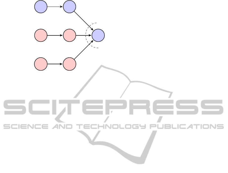
Figure 7: A path from the task t

to t

via task t

in the

task graph, the two copies of the tasks t

and t

denoted by

, t

and t

, t

respectively, and the delay random variable

D[t

, t

] for an edge (t

, t

) ∈ A.

4.1 Task Replication

The path delay constraints (3) depends on the con-

stants maxDelay and minProbability, which is pro-

vided by the developer as part of the task graph.

Therefore, it is possible that these constraints are not

satisﬁable. To tackle this issue, we replicate certain

tasks more than once in a region, for the express pur-

pose of reducing the possible delay values of the ran-

dom variables L[t

, t

] (since t

can ﬁre as soon as one

of the clones’ data is available). This will incur a

cost in terms of communication overhead. However,

we formulate the problem to minimise the number of

replicated tasks and hence minimise the communica-

tion overhead.

In Figure 7, we show an example of task replica-

tion on the path p

from the task t

to t

, with the

tasks t

, t

replicated from the task t

, and the tasks

, t

replicated from the task t

. A replicated task also

replicates the incoming and outgoing edges from the

direct predecessor and to the direct successor tasks in

the task graph. We only replicate the operational tasks

(namely t

and t

in Figure 7), and as a result the two

new paths p

and p

share the actuator task t

The latency for the delay at an end-point t

on the

path p

is equal to the minimum of the delay random

variable L of all paths p

, p

and p

L[t

, t

] = min



L[t

, t

], L[t

, t

], L[t

, t

]



In the general case, the delay random variable L[t

, t

]

along a path with the tasks replication is computed by

an additional operator = (operator min in our work,

which is provided by the probability model) to com-

pose the properties of the channels over the (parallel)

fan-in at the end-point task t

L[t

, t

] = =

) ∈ A

(L[t

, t

] ⊕ D[t

, t

]) (8)

where A

is the set of all replicated edges for the direct

predecessor of the task t

including the non-replicated

edge on the path from t

to t

Based on order statistics (Arnold et al., 2008;

David and Nagaraja, 2003), the c.d.f of L[t

, t

] in (8)

with the operator = being the minimum of indepen-

dent random variables becomes:

∀ t

∈ S, t

∈ E,

, t

] =

1 − (1 − F

, t

])· (1 − F

, t

])···(1 − F

, t

])

(9)

where t

represents the r

copy of the task t

For example, in Figure 7, we can use the equa-

tion (9) to compute the latency at the task t

. As-

sume on the path p

the tasks can only be placed on

different nodes (node[t

] 6= node[t

]), also

let maxDelay = 2, minProbability = 0.98, and the de-

lay distribution be normal distribution N(0.5, 1) for

all edges. From (7), before replicating the tasks, the

c.d.f F

, t

] of the delay random variable on path p

becomes:

node[t

] 6= node[t

] ∧ node[t

] 6= node[t

] =⇒

, t

] = Φ

0.5+0.5,1+1

= Φ

1,2

and the probability of the latency on the path p

being

at most 2.0 seconds is F

, t

](2) = 0.76025. How-

ever, 0.76025  0.98 and the constraint (3) is not sat-

isﬁable. In order to satisfy constraint (3), we create

two copies of the tasks t

and t

as shown in Figure 7.

The replicated tasks maintain the same properties and

the originated tasks. Hence, the probability of latency

being at most 2 seconds on path p

and p

is also

0.76025. Using equation (9) we have:

, t

] =

1−(1−0.76025)·(1−0.76025)·(1−0.76025) = 0.9862

and the constraint (3) is satisﬁed (0.9862 ≥ 0.98).

The task mapping optimisation problem with tasks

replication becomes:

minimise |T

subject to:

node[t] 6= n for every task t that

cannot be mapped to node n

(10)

∀ t

∈ S, t

∈ E,

, t

](maxDelay) ≥ minProbability

(11)

where T

is the set of all replicated tasks, and F

, t

]

is computed from (9).

AConstraintProgrammingApproachforManagingEnd-to-endRequirementsinSensorNetworkMacroprogramming

4.2 Task Replication Lower bound

For any given path p from the task t

to the task t

the mapping of all tasks to different nodes incurs the

maximum latency at the end-point task t

. Let MF be

the maximum latency incurred by assigning all tasks

to different nodes (MF = max (F

, t

])), and r be the

number of replicated tasks. The lower bound on the

number of tasks replicated is:

, t

] = 1 − (1 − MF)

≥ minProbability =⇒

(1 − MF)

≤ 1 − minProbability =⇒

r · log(1 − MF) ≤ log(1 − minProbability) =⇒

r ≥

log(1 − minProbability)

log(1 − MF)

(12)

For example, as we have shown in Figure 7 with

minProbability = 0.98 and MF = 0.76025, we require

to replicate the tasks on the path p

at least two times,

which can also be derived using the lower bound (12):

r ≥

log(1 − 0.98)

log(1 − 0.76025)

= 2.74121

In our implementation, we use the ﬂoor of the lower

bound in (12) to compute the minimum number of

replicated tasks required.

5 CONSTRAINT

PROGRAMMING APPROACH

FOR END-TO-END

REQUIREMENTS

As we have seen in Section 4, the abstract nature

of the path delay constraints (3) and the c.d.f of la-

tency (7) at an end-point being a piecewise function

of the decision variables node[t], make it very difﬁcult

to implement and solve the task mapping optimisation

problem with end-to-end requirements using conven-

tional approaches and optimisation solvers. In this

section, we use constraint programming (CP) to im-

plement the mathematical model stated in Section 4.

Algorithm 1 lists our CP approach in solving the

task mapping problem with delay requirements. In

our main CP model (CSP

main

in line 2), each path de-

lay constraint (3) is modelled as a sub constraint sat-

isfaction problem (CSP

sub

in line 8), and the whole

solution to each sub-CSP is expressed as an exten-

sional constraint (also known as user-deﬁned or ad-

hoc constraint). Extensional constraints provide a

way to specify all valid solutions to the constraint, us-

ing either a deterministic ﬁnite automaton or a tuple

set (table constraint). In this work, we use a tuple set

Algorithm 1: The task mapping with end-to-end

delay requirements algorithm.

input : N, T, S, E, minProbability

output: node

1 solved ← false

2 add placement constraints to CSP

main

3 while not solved do

4 taskCopiesRequired ← false

5 forall t

∈ S, t

∈ E do

6 tupleSet[t

, t

] ←

7 taskCopies ← 0

8 forall solutions s in CSP

sub

hp[t

, t

]i do

9 if checker(s, MF) then

10 tupleSet[t

, t

] =

tupleSet[t

, t

] ∪ s

11 if tupleSet[t

, t

] 6=

0 then

12 add extentsional constraints to

CSP

main

13 else

14 taskCopies ←

log(1−minProbability)

log(1−MF)

15 replicate(p[t

, t

], taskCopies)

16 taskCopiesRequired ← true

17 if not taskCopiesRequired then

18 solve(CSP

main

)

19 if CSP

main

has a solution then

20 solved ← true

21 return node

22 else

23 replicate (1)

to express all the valid solutions to the path delay con-

straints (3) and enforce these constraints in our main

CP model.

Our CSP

main

model enforces the placement con-

straints (1) and the following extensional constraint

representing the valid solutions to the path delay con-

straints (3):

∀ t

∈ S, t

∈ E

extensional(p[t

, t

], tupleSet[t

, t

])

(13)

where p[t

, t

] is the set of all tasks on the path from

the task t

to the task t

including t

and t

, and

tupleSet[t

, t

] is the set of tuples, where each tuple

is a valid solution to the path delay constraint (3),

given by solving the CSP

sub

(line 8). The extensional

constraints (13) are then constraining the valid solu-

tions of the path delay constraints to the correspond-

ing variables node[t], t ∈ p[t

, t

] (line 12), on which

domain consistency (all values not participating in a

SENSORNETS2014-InternationalConferenceonSensorNetworks

solution are pruned) is achieved.

For example, in Figure 5, let the delay random

variable D be a normal distribution N(0.5, 1), and the

domain of the tasks be as follows:

node[t

] = {1, 2}, node[t

] = {2}

also let maxDelay = 3, minProbability = 0.98. The

path delay constraints according to (7) become:

, t

] =











F(D; 0) if node[t

, t

] = [3, 3, 3]

0.5,1

if node[t

, t

] = [2, 3, 3]

0.5,1

if node[t

, t

] = [2, 2, 3]

1,2

if node[t

, t

] = [3, 2, 3]

(14)

where node[t

, t

] = [3, 3, 3] is a vector notation for

the assignment node[t

] = 3, node[t

] =

3. The path delay constraints (3) for all the possible

assignments in (14) become:

node[t

, t

] = [3, 3, 3] =⇒

, t

](3) = F(D; 0) = 1 ≥ 0.98 (15)

node[t

, t

] = [2, 3, 3] =⇒

, t

](3) = Φ

0.5,1

(3) = 0.99379 ≥ 0.98 (16)

node[t

, t

] = [2, 2, 3] =⇒

, t

](3) = Φ

0.5,1

(3) = 0.99379 ≥ 0.98 (17)

node[t

, t

] = [3, 2, 3] =⇒

, t

](3) = Φ

1,2

(3) = 0.92135  0.98 (18)

The possible assignments (15), (16), and (17) sat-

isfy the path delay constraint, except the assign-

ment node[t

, t

] = [3, 2, 3] (18). Note that the

tupleSet[t

, t

] only includes valid assignments:

tupleSet[t

, t

] = {[3, 3, 3], [2, 3, 3], [2, 2, 3]}

and therefore in this example the extensional con-

straint (13) is:

extensional({t

, t

}, {[3, 3, 3], [2, 3, 3], [2, 2, 3]})

(19)

The extensional constraint (19) constrains the deci-

sion variables node[t

], node[t

], and node[t

] to the

given valid assignments by the tupleSet. In the pres-

ence of many extensional constraints for several path

delay constraints, our CSP

main

model can effectively

prune the values that do not participate in a solution,

using the produced valid assignments tupleSet given

by the CSP

sub

model.

The CSP

sub

model produces solutions to the

ground instance of the task mapping problem with

only decision variables limited to one path on the

task graph, and only includes placement constraints.

Therefore, it is efﬁcient to produce all solutions and

check the validity of each solution using a checker

function (line 9). The checker function computes

the c.d.f of the delay according to (9) and incremen-

tally maintains the maximum value of the c.d.f (MF)

to be used in computing the lower bound taskCopies

on the tasks replication (line 14). The checker func-

tion returns true if in the assignment s the c.d.f of the

delay is at least minProbability satisfying the path de-

lay constant (3), and false otherwise. If the checker

function returns true, the valid solution s is added to

the tupleSet[t

, t

] (line 10), and if there is at least one

valid solution (tupleSet[t

, t

] 6=

0, line 11), then the

extensional constraint (13) is added to the CSP

main

model (line 12). Note that the initial domain reduc-

tion is performed by the extensional constraints at this

point (all values not participating in a solution to the

CSP

main

are pruned from the domains of the decision

variables), which reduces the number of solutions for

the consecutive CSP

sub

models.

If there is no valid solution to CSP

sub

(tupleSet[t

, t

] =

0, line 13), then at least one of

the path delay constraints can not be satisﬁed, hence

CSP

main

is also not satisﬁable, and we required to

replicate the tasks. We replicate the tasks such that

the path delay constraints over the path p are satisﬁed,

and we start from the mathematical lower bound on

the number of task copies taskCopies (line 14). The

replicate function (line 15) takes the path p[t

, t

]

and creates taskCopies replicates of the operational

tasks along the path maintaining the same incoming

and outgoing edges in the path p[t

, t

] from the task

graph.

We solve CSP

main

(line 20) only if all path

delay constraints are individually satisﬁable

(no task replicate per path basis is required,

taskCopiesRequired = false, line 17). If CSP

main

has

a solution, the node decision variables are returned

(line 21) and the algorithm ends, otherwise CSP

main

became unsatisﬁable due to the composition of all

path delay constraints, therefore we add one more

copy of each operational tasks in the task graph G

(line 23).

We further optimise the CSP

sub

model by adding

symmetry breaking constraints (Rossi et al., 2006).

Let p

, t

] be the k

set of replicated tasks on the

path from t

to t

, where p

, t

] represents the initial

tasks from t

to t

. We refer to p

, t

] as the k

repli-

cated path. Let v

, t

] be the vector of the decision

variables node[t] on the k

replicated path in the or-

der of the directed edges. We enforce lexicographic

ordering to remove the equivalent permutation of val-

ues in a solution to CSP

sub

between replicated paths,

AConstraintProgrammingApproachforManagingEnd-to-endRequirementsinSensorNetworkMacroprogramming

where there is at least one replicated path required:

∀p

, t

], 0 ≤ k ≤ NR[t

, t

]

, t

] 

lex

k+1

, t

]

(20)

where NR[t

, t

] is the number of replicated paths from

task t

to t

and 

lex

is the lexicographic ordering

constraint between the vectors of decision variables

, t

] and v

k+1

, t

6 EVALUATION

6.1 Experimental Setup

In our experiments, we use the realistic road trafﬁc

application and its latency requirements in (US De-

partment of Transportation, Federal Highway Admin-

istration, 2012). We start from the smallest highway

trafﬁc size of h|N|, |T|i = h7, 9i and increase the in-

stance size by one region per instance (each region is

a sector in a highway with at least 6 sensor nodes)

up to the largest instance of highway trafﬁc with 25

regions (highway trafﬁc h150, 216i). We assume that

the delay distribution for sending a message between

any two regions is a normal distribution N(0.5, 1)

with mean 0.5 and variance 1. For each instance, we

enforce the end-to-end delay constraints between the

AverageSpeedCalculator tasks and the RampSignalD-

isplayer tasks with the message delay probability of

0.98 within 1, 2, or 3 seconds.

Our CP model is implemented in Gecode (Gecode

Team, 2006) (revision 4.2.0)

and runs under

Mac OS X 10.8.4 64 bit on an Intel Core i5 2.6 GHz

with 3MB L2 cache and 8GB RAM. We separately

solve each instance for the maximum delay value

(maxDelay) of 1, 2, or 3 seconds. We set a timeout

of 60 seconds for each instance, recording the time to

solve optimally and the number of replicated tasks.

6.2 Analysis of Results

In Figure 8, we present the average runtime results (in

seconds) of 10 runs for solving the highway trafﬁc in-

stances with our CP model. Each instance is solved

upon varying the delay requirement (maxDelay) on

the values 1, 2, and 3 seconds. The lower values

of maxDelay makes the instances more difﬁcult to

solve, as the delay requirement becomes harder to

satisfy and more task replicates are required. All in-

stances were solved optimally, minimising the num-

ber of replicated tasks.

available from http://www.gecode.org/

0.0001

0.001

0.01

0.1

h7, 9i

h13, 18i

h19, 27i

h25, 36i

h32, 45i

h38, 54i

h44, 63i

h50, 72i

h57, 81i

h63, 90i

h69, 99i

h75, 108i

h82, 117i

h88, 126i

h94, 135i

h100, 144i

h107, 153i

h113, 162i

h119, 171i

h125, 180i

h132, 189i

h138, 198i

h144, 207i

h150, 216i

Runtime (seconds)

Highway traﬃc instances

maxDelay = 1

maxDelay = 2

maxDelay = 3

Figure 8: Average runtime in seconds of 10 runs and in log-

arithmic scale for solving optimally the task mapping prob-

lem with end-to-end requirements on the highway trafﬁc ap-

plication with a maximum allowed delay of 1, 2, or 3 sec-

onds. The instances are represented with h|N|, |T|i, where

|N| is the number of sensor nodes and |T| is the number of

instantiated tasks.

100

150

200

250

300

350

h7, 9i

h13, 18i

h19, 27i

h25, 36i

h32, 45i

h38, 54i

h44, 63i

h50, 72i

h57, 81i

h63, 90i

h69, 99i

h75, 108i

h82, 117i

h88, 126i

h94, 135i

h100, 144i

h107, 153i

h113, 162i

h119, 171i

h125, 180i

h132, 189i

h138, 198i

h144, 207i

h150, 216i

Replicated tasks

Highway traﬃc instances

maxDelay = 1

maxDelay = 2

maxDelay = 3

Figure 9: Number of replicated tasks required to satisfy the

end-to-end requirements on the highway trafﬁc application

with a maximum allowed delay of 1, 2, or 3 seconds. The

instances are represented with h|N|, |T|i, where |N| is the

number of sensor nodes and |T| is the number of instantiated

tasks.

The runtimes for instances with maxDelay = 2 and

3 seconds are very short, therefore we take the aver-

age runtime of 10 runs. In Figure 8, we present the

runtimes with logarithmic scale to further distinguish

the difference of runtime between the instances with

maxDelay = 2 and instances with maxDelay = 3 sec-

onds. The runtime includes the preprocessing time to

create and solve the CSP

sub

models, and the runtime

to solve the CSP

main

model. The runtime increases

linearly as the size of the problem increases and the

maximum allowed delay (maxDelay) decreases. For

the ﬁrst instance h7, 9i, the runtime is signiﬁcantly

shorter than larger instances, because this instance in-

volves only one region with one path delay constraint,

and requires only 2 task replicates to satisfy the de-

SENSORNETS2014-InternationalConferenceonSensorNetworks

0.001

0.01

0.1

100

1000

0.7 0.8 0.9 1.0 1.2 1.4 1.6 1.8 2 4 8 16 32

Runtime (seconds)

maxDelay

Highway traﬃc instance h132, 189i

Figure 10: The average runtime in seconds and logarithmic

scale for solving highway trafﬁc instance h132, 189i with

10 runs, varying maxDelay.

lay requirement when maxDelay = 1 or 2 seconds.

The runtime drastically increases as the maximum al-

lowed delay drops below the average delay on a path

between two end-points with delay requirements. In

our instances, the paths between the two end-points

includes three edges (path length is 3), where the

average delay on each edge is 0.5 second, therefore

the average delay between the two end-points on the

path is 1.5 seconds, and choosing maxDelay = 1 sec-

ond requires several iterations of creating task repli-

cates, hence the longer runtimes. The standard de-

viation of the runtimes for all instances is on average

0.05 seconds, and at most 1.69 seconds, while varying

maxDelay between 1 and 3 seconds with 10 runs.

In Figure 9 we present the number of replicated

tasks in order to satisfy the end-to-end requirements

expressed by the path delay constraints in our CP

model. As we expected, a tighter requirement on the

allowed maximum delay (maxDelay) requires more

replicated tasks to improve the chance of a message

delivery at an end-point and to satisfy the path de-

lay constraints. As the delay requirement maxDelay

drops from 2 seconds to 1 second, the replicated tasks

are not exactly doubled, as some path delay con-

straints are satisﬁed with fewer replicated tasks. How-

ever, increasing the instance size by one region in-

creases the number of task replicates equally between

two consecutive instances, which is due to the equal

delay distribution between all regions.

In Figure 10, we present the average runtime re-

sults (in seconds) of 10 runs for solving a reason-

ably large instance of the highway trafﬁc application

(namely instance h132, 189i), varying the values of

maxDelay from 0.7 to 32 seconds. In Figure 11, we

show the results for the number of replicated tasks

with the same setup as in Figure 10. The result shows

that the runtime and the number of replicated tasks

follow the same trend, while varying the maximum al-

100

150

200

250

300

350

400

450

0.7 0.8 0.9 1.0 1.2 1.4 1.6 1.8 2 4 8 16 32

Replicated tasks

maxDelay

Highway traﬃc instance h132, 189i

Figure 11: Number of replicated tasks required to satisfy

the end-to-end requirements on the highway trafﬁc instance

h132, 189i, varying maxDelay.

lowed delay maxDelay. The runtime tightly depends

on the number of replicated tasks, and there is an in-

terval on the values of maxDelay, where the average

runtime and the number of replicated tasks does not

change signiﬁcantly.

These results show that constraint programming

can efﬁciently solve the combinatorial problem with

end-to-end requirements introduced in task mapping

for WSNs.

7 CONCLUSIONS

In this paper, we formulated the problem as a con-

straint program of task-mapping while honouring

end-to-end requirements encountered during sensor

network macroprogramming, and presented efﬁcient

algorithms to solve it. We also addressed the case

when copies of certain tasks are permitted in or-

der to increase performance guarantees. Our evalu-

ations, performed on a realistic highway trafﬁc ap-

plication task graph for the special case of manag-

ing end-to-end latency, show that this problem can

indeed be solved efﬁciently using our approach, al-

though increased computation time is needed for

tighter bounds. We investigated the speciﬁc case of

latency requirement in this paper. However the end-

to-end requirements are only given as an example. It

is possible to address other end-to-end requirements

by changing the rules of the probability model for

combining the probability distributions along the path

between the two end points. For example, if instead of

latency we consider link quality as a random variable

over the channels, then the probability model must

state the distribution of the random variable link qual-

ity and how it is combined over channels (path be-

tween two end-points). We then replace the operator

AConstraintProgrammingApproachforManagingEnd-to-endRequirementsinSensorNetworkMacroprogramming

⊕ and = (8) in the the probability model with the op-

erator product and the operator min, respectively, and

our formulation (see Section 4) is still valid for main-

taining the link quality requirements. Our immediate

future work is in two parallel directions: i) integra-

tion of our approach into the publicly available Srijan

toolkit

for ATaG, and ii) further exploring the over-

head induced by creating copies of tasks and devel-

oping more accurate CP models to minimise it while

achieving the desired non-functional guarantees. We

also envision the application of our work in cloud

computing and related technologies, where guaran-

teeing certain requirements on the services running in

the cloud is essential, and latencies among co-located

nodes are similar to those in different data centres.

ACKNOWLEDGEMENTS

This research is partially sypported by the Swedish

Foundation for Strategic Research (SSF) under re-

search grant RIT08-0065 for the project ProFuN,

and the French ANR-BLAN-SIMI10-LS-100618-6-

01 MURPHY project. Special thanks to the reviewers

for their comments.

REFERENCES

Arnold, B. C., Balakrishnan, N., and Nagaraja, H. N.

(2008). A ﬁrst course in order statistics, volume 54 of

Classics in Applied Mathematics. Society for Indus-

trial and Applied Mathematics (SIAM), Philadelphia,

PA. Unabridged republication of the 1992 original.

Bakshi, A., Pathak, A., and Prasanna, V. K. (2005a).

System-level support for macroprogramming of net-

worked sensing applications. In Intl. Conf. on Perva-

sive Systems and Computing (PSC).

Bakshi, A., Prasanna, V. K., Reich, J., and Larner, D.

(2005b). The Abstract Task Graph: A methodol-

ogy for architecture-independent programming of net-

worked sensor systems. In Workshop on End-to-end

Sense-and-respond Systems (EESR).

Choi, W., Shah, P., and Das, S. (2004). A framework for

energy-saving data gathering using two-phase cluster-

ing in wireless sensor networks. In Proc. of the 1

Int.

Conf. on Mobile and Ubiquitous Systems: Networking

and Services (MOBIQUITOUS).

David, H. A. and Nagaraja, H. N. (2003). Order statis-

tics. Wiley Series in Probability and Statistics. Wiley-

Interscience [JohnWiley & Sons], Hoboken, NJ, third

edition.

Gecode Team (2006). Gecode: A generic constraint devel-

opment environment. http://www.gecode.org/.

http://code.google.com/p/srijan-toolkit/

Gummadi, R., Gnawali, O., and Govindan, R. (2005).

Macro-programming wireless sensor networks using

Kairos. In Proc. of the 1

Int. Conf. on Distributed

Computing in Sensor Systems (DCOSS).

Hassani Bijarbooneh, F., Flener, P., Ngai, E., and Pearson, J.

(2011). Energy-efﬁcient task mapping for data-driven

sensor network macroprogramming using constraint

programming. In Operations Research, Computing,

and Homeland Defense, pages 199–209. Institute for

Operations Research and the Management Sciences.

Karr, A. (1993). Probability. Springer Texts in Statistics

Series. Springer-Verlag.

Mottola, L., Pathak, A., Bakshi, A., Prasanna, V. K., and

Picco, G. P. (2007). Enabling scope-based interactions

in sensor network macroprogramming. In Proc. of the

4th Int. Conf. on Mobile Ad-Hoc and Sensor Systems.

Mottola, L. and Picco, G. (2011). Programming wireless

sensor networks: Fundamental concepts and state of

the art. ACM Computing Surveys (CSUR), 43(3):19.

Newton, R., Morrisett, G., and Welsh, M. (2007). The reg-

iment macroprogramming system. In Proceedings of

the 6th international conference on Information pro-

cessing in sensor networks, pages 489–498. ACM.

Pathak, A., Mottola, L., Bakshi, A., Prasanna, V. K., and

Picco, G. P. (2007). Expressing sensor network inter-

action patterns using data-driven macroprogramming.

In Third IEEE International Workshop on Sensor Net-

works and Systems for Pervasive Computing (PerSeNS

2007).

Pathak, A. and Prasanna, V. K. (2010). Energy-efﬁcient

task mapping for data-driven sensor network macro-

programming. IEEE Transactions on Computers,

59(7):955–968.

Pathak, A. and Prasanna, V. K. (2011). High-Level Applica-

tion Development for Sensor Networks: Data-Driven

Approach. In Nikoletseas, S. and Rolim, J. D., editors,

Theoretical Aspects of Distributed Computing in Sen-

sor Networks, Monographs in Theoretical Computer

Science. An EATCS Series, pages 865–891. Springer

Berlin Heidelberg.

Rossi, F., van Beek, P., and Walsh, T., editors (2006). Hand-

book of Constraint Programming. Elsevier.

Tian, Y., Ekici, E., and

Ozg

uner, F. (2005). Energy-

constrained task mapping and scheduling in wireless

sensor networks. In IEEE International Conference

on Mobile Ad hoc and Sensor Systems, pages 8–218.

IEEE Computer Society Press.

US Department of Transportation, Federal Highway Ad-

ministration (2012). Manual on uniform trafﬁc con-

trol devices: Preemption and priority control of

trafﬁc control signals. http://mutcd.fhwa.dot.gov/

pdfs/2009r1r2/part4.pdf. Section 4D.27.

Wu, Y., Kapitanova, K., Li, J., Stankovic, J. A., Son, S. H.,

and Whitehouse, K. (2010). Run time assurance of

application-level requirements in wireless sensor net-

works. In Proceedings of the 9th ACM/IEEE Interna-

tional Conference on Information Processing in Sen-

sor Networks, IPSN ’10.

SENSORNETS2014-InternationalConferenceonSensorNetworks