
A Study of Channel Classification Agreement in Urban Wireless Sensor
Network Environments
Aikaterini Vlachaki, Ioanis Nikolaidis and Janelle Harms
Computing Science Department, University of Alberta, Edmonton, T6G 2E8, Alberta, Canada
Keywords:
Wireless Sensor Networks (WSNs), Cognitive Networking, Sample Cross-correlation, Received Signal
Strength Indicator (RSSI), Channel State.
Abstract:
We consider a wireless sensor network in an urban environment and attempt to characterize the interference
found in the communication channel by means of empirically collected Received Signal Strength Indicator
(RSSI) values over Industrial, Scientific and Medical (ISM) and non-ISM bands. We assume a node-based
interference classification scheme exists and examine whether nodes that classify the channel as belonging
to the same class also exhibit strong cross-correlation in terms of the RSSI time series they independently
observe. In effect, we are studying how the agreement of nodes, e.g., via consensus, on the class of a channel
can be linked to the cross-correlation statistic and to what extent. We find that the particular class impacts the
degree to which we can confidently claim that the channel observed independently by each node, and classified
to belong to the same class, indeed behaves the same way.
1 INTRODUCTION
It is often asserted that Wireless Sensor Networks
(WSNs) will be increasingly deployed in hostile envi-
ronments. While hostile environment usually means
an environment inhospitable to human presence, in
another sense a hostile environment can be one of
continuous human presence albeit with adverse im-
pact on the operation of the WSN nodes. Such is
the case of urban environments with the multitude
of sources of interference, some of which are rather
well-understood, e.g., other co-located wireless data
communication networks, and some that are less so,
i.e., electromagnetic interference from nearby oper-
ating appliances (lamps, microwaves, etc.), elevators,
car engines, etc. It is tempting to lump all such inter-
ference into a category that, on the average and across
a large number of interferers, would be conveniently
modelled as a Gaussian noise source. Unfortunately,
empirical evidence collected so far (Lee et al., 2007;
Boers et al., 2010) suggest that interference in urban
environments does not fit the simplifying Gaussian
assumption.
In this study we extend a previous effort of char-
acterizing the background interference in a deployed
WSN (Boers et al., 2010). The benefits of being able
to characterize the interference should be obvious be-
cause, for example, it would allow the operation of
the WSN to adopt strategies to circumvent the in-
terference and its impact. A Media Access Control
(MAC) protocolthat operatesaround interference pat-
terns was developed (Boers et al., 2012a) but it is only
an example of a broader set of options available to the
designer. In general, the presented work is related to
the area of cognitive networking. However, it is the
restricted nature of the abilities of the nodes that drive
the presented research. Namely, we assume that the
nodes have only a single means, a signal strength in-
dicator, for sensing the channel for purposes of ana-
lyzing any interference patterns. No special support
from the physical layer is assumed or required.
Specifically, we study interference in urban envi-
ronments to test whether the often–assumed strategy
of deriving a distributed consensus across nodes as to
the nature of the channel is a strategy that reflects the
reality of the channel. In consensus strategies, each
node independently classifies the channel based on its
own measurements and provides the result of its clas-
sification to the rest of the nodes. Subsequently, and
depending on the formation of consensus, decisions
about the use (or not) and the exact technique to ac-
cess the channel can take place. We are not interested
in the decisions taken after the consensus is reached
but on whether the channel indeed behaves the same
way from the viewpoint of the nodes that determined
the channel behavior to belong to the same class. For
249
Vlachaki A., Nikolaidis I. and Harms J..
A Study of Channel Classification Agreement in Urban Wireless Sensor Network Environments.
DOI: 10.5220/0004716102490259
In Proceedings of the 3rd International Conference on Sensor Networks (SENSORNETS-2014), pages 249-259
ISBN: 978-989-758-001-7
Copyright
c
2014 SCITEPRESS (Science and Technology Publications, Lda.)

example, if a node detects a periodic spike of inter-
ference sufficient to classify it as a channel with peri-
odic interferer, it might agree with the class identified
on the same channel by another node, but there is no
guarantee that the two nodes sense the same periodic
interferer.
The model assumed throughout this paper is that
each node independently decides on what is the na-
ture of the interference via a classification technique
(placing it in one of five classes) as outlined in (Boers
et al., 2010). To facilitate a comparison of the back-
ground interference as seen by different nodes, we
develop a technique to correct the lack of synchro-
nization across the samples collected by the differ-
ent nodes. The lack of synchronization is caused by
the absence of a global clock and the individual node
clock drift. The purpose of the paper is to study, from
collected empirical evidence whether, if, when con-
sensus is reached, it is indeed valid, i.e., it concerns
the same interferenceseen by all the nodesat the same
points in time. To this end, we examine whether, if
consensus exists, the levels of interference are com-
patible across the nodes, i.e., the small time scale
behavior is the same. For example two nodes with
a valid consensus characterizing the channel as hav-
ing periodic spikes may still perceive different noise
floors and variance of noise between spikes, making
the potential Signal to Noise Ratio (if a transmission
were to be attempted) drastically different from the
perspective of the two nodes. In short, we are study-
ing whether a simple class-based consensus can be re-
lied upon to represent the common reality across the
nodes of the same WSN.
The rest of the paper is organized as follows. In
Section 2, we review the related literature. In Sec-
tion 3, we investigate and present the data we use in
our study. Section 4 explains the methodologywe fol-
low to analyze the data. Our results are presented in
Section 5. Section 6 provides concluding remarks.
2 RELATED WORK
Researchers studying the impact of external interfer-
ence in urban environments concentrate on identify-
ing and classifying patterns of noise and interference,
as well as applications of related classification tech-
niques to cognitive networking.
Lee, Cerpa and Lewis (Lee et al., 2007) measure
noise traces in many different environments in order
to propose algorithms to simulate noise and interfer-
ence. From these traces they observed three main
patterns of interference, (i) rapid spikes, (ii) periodic
spikes and (iii) noise patterns changing over time.
Boers, Nikolaidis and Gburzynski (Boers et al.,
2010) measured noise and interference in a four-by-
four node WSN, at high sample rates. They ex-
tracted five dominant noise and interference patterns:
(i) quiet, (ii) quiet with spikes, (iii) quiet with rapid
spikes, (iv) high and level and the (v) shifting mean
pattern. Consequently, they classified them using a
Bayesian network classifier. Later, this work was ex-
tended by classifying two of the aforementioned pat-
terns locally at each node using single-node decision
tree classifiers (Boers et al., 2012b).
In cognitive-networking, known identified pat-
terns can be exploited to coordinate cooperative sens-
ing across the nodes of a WSN. The determined
noise and interference patterns for each WSN can be
utilized to build a distributed classifier. In such a
scheme, the WSN nodes cooperate with each other
to reach a consensus on a specific pattern, after a
number of iterations, by exchanging and combining
their sensing information. This aims to eliminate
the impact of deficient individual pattern classifica-
tions (Akyildiz et al., 2011). The notion of coopera-
tive sensing extends also to multi-hop cases whereby
the sensing results of nodes are forwarded over mul-
tiple hops in order to improve the classification accu-
racy.
Rather than develop a scheme that attempts to
combine sensed measurements from the nodes to
reach a classification result, we examine whether indi-
vidual per-node classification and a simple network-
wide consensus is sufficiently accurate, at least in
WSN networks deployed in a small space such as the
network that is the object of this study. Per–node clas-
sification is justified because we wish to generate con-
sensus (and possibly revise it over time) without un-
due burden on the sensor nodes in terms of transmis-
sions. The alternative would have been the collection
of background noise signal strength data from all the
nodes to a host/sink that performs elaborate computa-
tion to decide on the state of the channel. Clearly,
the collection of all background noise and interfer-
ence samples to a sink is unattractive as it represents
a high energy cost to transmit them. Instead, we con-
sider an architecture whereby each WSN node classi-
fies, in isolation, the state of the channel and then a
consensus is derived using a message from each node
that indicates just the determined class, hence reduc-
ing the volume of data that need to be exchanged.
3 THE DATA
In this study, we use the RSSI traces collected by
Boers et al. (Boers et al., 2010), across 256 chan-
SENSORNETS2014-InternationalConferenceonSensorNetworks
250

Figure 1: The experimental setup within the Smart Condo.
The circles represent the WSN nodes. The computer col-
lecting the data was placed outside the grid of WSN nodes
(top-left) (Boers et al., 2010).
nels spanning ISM and non-ISM bands in an indoor
urban environment. We concentrate on the sample-
cross correlation for each channel and for every pair
of nodes, aiming to quantify and justify the similar-
ity between nodes that have classified the channel as
exhibiting the same pattern, as well as to identify dis-
agreements at a microscopic level.
3.1 The Data Collection System
The RSSI traces were collected within the first imple-
mentation of the Smart Condo at the University of Al-
berta within the Telus Centre (a medium sized office
building) at the University of Alberta, located across
from a large residential apartment building (Boers
et al., 2009). Within the 80 m
2
space of the Smart
Condo, WSN nodes were placed in a four-by-four
grid with 1.84 m spacing as presented in Fig.1. Each
node stood 28 cm above floor level. While running the
data collection experiments, the room’s doors were
closed and there was no movement within the room.
Additionally, all the measurements were noise mea-
surements, meaning that the sensor nodes did not in-
troduce any transmissions on their own.
The WSN nodes were model EMSPCC11 pro-
vided by Olsonet Communications (Olsonet, 2008)
consisting of a TI MSP430F1611 microcontroller
and a TI CC1100 transceiver. The transceiver was
configured for 38.4 kbit/s using 2-FSK modula-
tion. The nodes ran an operating system named Pi-
cOS (Akhmetshina et al., 2003) and a PicOS appli-
cation collected noise measurements by reading the
RSSI value from the CC1100’s RSSI register.
The RSSI was measured by each one of the 16
nodes of the WSN for every channel. In total, 256
channels were examined to produce a total of 4096
traces. The configuration of the WSN nodes was at
a base frequency of 904 MHz. The channels were
spaced 199.9512 kHz apart. Each channel occupies a
bandwidth of 101.5625 kHz. Using these settings the
nodes were listening on frequencies within and out-
side the ISM band, from 904 MHz to 928 MHz and
929 MHz to 954 MHz, respectively. For each chan-
nel and node combination 175000 successive RSSI
samples were collected, representing a duration of 35
seconds. The entire data collection process was com-
pleted in approximately 2.5 hours.
3.2 Channel Classes
As described in Section 2, five dominant noise and
interference patterns were encountered from a closer
examination and the hand classification of the col-
lected RSSI traces. We repeat here the characteristics
of each class:
1. The quiet channel, which is characterized by a low
maximum.
2. The quiet-with-spikes channel is similar to the
quiet channel, but it has short-duration spikes that
give it a higher maximum.
3. The quiet-with-rapid-spikes channel has a higher
frequency of spikes than the quiet-with-spikes
channel.
4. The high-and-level channel exhibits a high and
tight level and has a high minimum.
5. The shifting-mean channel has its RSSI samples
distributed bimodally.
A visual classification of the noise traces for each
node per channel are presented in Fig. 2.
4 THE METHODOLOGY
4.1 Pre–processing
Two significant parameters taken into consideration
are the node clock drifts and timestamping of the sam-
pled data, as well as the noisy nature of the RSSI
traces themselves.
4.1.1 Data Collection Timestamping
In Boers’ et al. work (Boers et al., 2010) the node
clock drift during the collection of the RSSI traces
was surprisingly high, even over short intervals. Since
WSN node clocks cannot be relied upon to provide
the correspondence to the natural time, the times-
tamping was performed with respect to the clock
of the personal computer to which the data collec-
tion was being streamed (via serial USB connections)
AStudyofChannelClassificationAgreementinUrbanWirelessSensorNetworkEnvironments
251
from the individual WSN nodes. In other words, the
clock of the collecting host was trusted as authorita-
tive. Naturally, this collection at the host was per-
formed for the purposes of the data analysis presented
here and is, in principle, absent in a real network. Be-
tween two readings from the same node/port several
RSSI samples could have been buffered in the mean-
time. In the case of multiple samples found in the
incoming buffer, the reading application would as-
sign those samples equi-spaced timestamps between
the current time and the time the buffer was read last.
The result is that two readings performed at the same
point in natural time from two differentnodes may ap-
pear with different timestamps. Hence, some means
of synchronizing the time series is necessary.
4.1.2 Re-sampling
We are creating a new set of time series consisting
of samples that all have (the same) specific times-
tamps. In this way, after the calculation of the sam-
ple cross-correlation the identification of similarity
(or not) of two series and the possible lagged rela-
tionship between them is going to be evident and re-
liable. Specifically, each RSSI time series (by a spe-
cific host at a specific channel) is 175000 values long.
The host application produced increasing timestamps
in the [0,35] secs interval. The re-sampling assigns
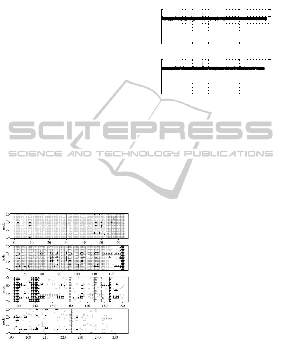
Figure 2: Classification of noise and interference traces
from 256 channels with 16 nodes per channel. The cor-
respondence between symbol and classification is: (a)
no symbol: quiet, (b): quiet with spikes, (c): quiet
with rapid spikes (d)H: high- and- level, (e)N: shifting
mean (Boers et al., 2010).
0 5 10 15 20 25 30 35
0
50
100
150
200
250
timestamp (secs)
Unsampled RSSI Time Series
RSSI value
0 5 10 15 20 25 30 35
0
50
100
150
200
250
timestamp (secs)
Re−sampled RSSI Time Series
RSSI value
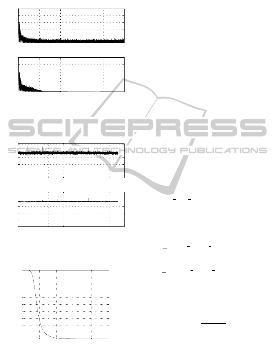
Figure 3: The RSSI time series from node 5 on channel 32
before and after re–sampling.
to samples a new timestamp in the same range [0, 35]
secs spaced 0.001 sec apart. Hence, the resulting re-
sampled trace will consist of 35000 values (corre-
sponding to timestamp “ticks” 0,0.001,0.002,...,35).
The re-sampled series includes the samples of the
original sequence that are closest (in terms of abso-
lute timestamp difference) to each tick. The deci-
sion to use the particular timestamp spacing of 0.001
secs results in ignoring several samples of the origi-
nal sequence but it was determined experimentally as
adequate because it did not result in the removal of
the features, e.g., spikes, that characterized each se-
ries. Larger timestamp granularities, e.g., 0.01 secs,
would not have left the features intact. For example,
in cases of channels presenting a quiet with spikes or
quiet with rapid spikes pattern, sampling at granulari-
ties of 0.01 secs or larger would have resulted in quiet
channels. As an illustration, Fig. 3 presents the RSSI
time series from channel 32 and node 5, that exhibits a
quiet–with–spikes pattern. It is evident that the signal
preserves its pattern before and after the re-sampling
as the spikes are all captured and coincide in the orig-
inal and the re-sampled series.
4.1.3 Filtering
The second step before the sample cross-correlation
estimation is to apply a low pass filter to the time se-
ries. This is done in order to enhance the calculation
of the cross-correlation by removing high–frequency
noise from the RSSI time series, leaving the charac-
teristic low–frequency shape of each sequence intact.
A low pass filter emphasizes the behaviour and the
characteristics of the observed patterns by producing
a time series where the amplitude of variations at high
frequencies is reduced.
SENSORNETS2014-InternationalConferenceonSensorNetworks
252
0 100 200 300 400 500
0
0.2
0.4
0.6
0.8
1
Single−Sided Amplitude Spectrum of x(t)
Frequency (Hz)
|X(f)|
0 100 200 300 400 500
0
0.2
0.4
0.6
0.8
1
Single−Sided Amplitude of filtered Spectrum of x(t)
Frequency (Hz)
|X(f)|
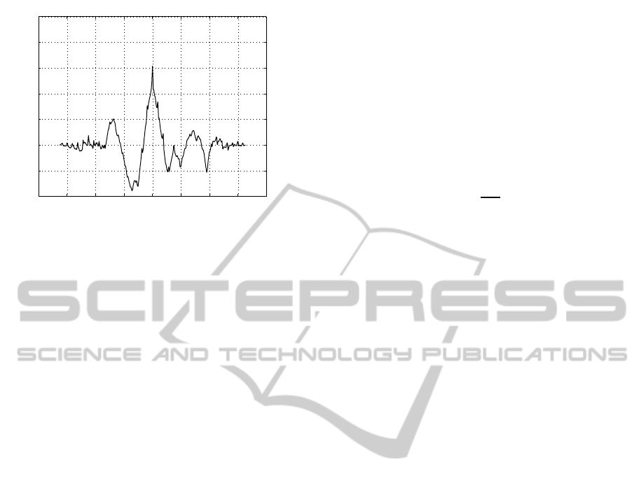
Figure 4: Frequency response of the RSSI time series from
channel 32 and node 5, before and after the application of
a Butterworth filter of 4th order with cutoff frequency 150
Hz.
0 5 10 15 20 25 30 35
0
50
100
150
200
250
timestamp (secs)
Re−sampled RSSI Time Series
RSSI value
0 5 10 15 20 25 30 35
0
50
100
150
200
250
timestamp (secs)
Filtered Re−sampled RSSI Time Series
RSSI value
Figure 5: Example of the application of the Butterworth
filter on the sampled RSSI time series from channel 32 and
node 5.
0 0.2 0.4 0.6 0.8 1
0
0.1
0.2
0.3
0.4
0.5
0.6
0.7
0.8
0.9
1
Frequency response of the filter
Gain
Normalized frequency (f/fo)
Figure 6: The frequency response of the Butterworth filter,
of 4th order, with cutoff frequency 150 Hz.
Namely, we apply, to each time series, a Butter-
worth low-pass filter of 4th order with a cut-off fre-
quency of 150 Hz (for a sample rate of 1000 Hz).
Its frequency response is presented in Fig. 6 and the
spectrum of a time series before and after the applica-
tion of this filter is presented in Fig. 4. Respectively,
we present in Fig. 5 the time series from channel 32
at node 5 before and after the filtering process. It is
evident that the low-frequency variations (spikes in
the case of Fig. 5) that are the feature characterizing
this time series, are preserved albeit with a somewhat
smaller amplitude. On the other hand, the high fre-
quency variations are smoothed out as expected.
4.2 Processing
In this section, we present the definition of sample
cross-correlation followedby the definition of another
tool, the Fano factor, that are helpful in examining
the relation of pairs of time series. We determine the
sample cross-correlation on all pairs of nodes and for
each channel.
4.2.1 Sample Cross-Correlation
The sample cross-correlation is a measure of similar-
ity of two time series as a function of a time-lag, or
time offset, between them. Consider N pairs of ob-
servations on two time series x
t
and y
t
where N is the
series length,
x and y are the sample means, and k is
the lag. The sample cross-covariance function (ccvf)
is given by (1) and (2). The sample variances of the
two series, c
xx
and c
yy
are described by (3) and the
sample cross-correlation is given by (4).
c
xy
(k) =
1
N
N−k
∑
t=1
(x
t
−
x)(y
t+k
−y), k = 0,1,..., (N −1) (1)
c
xy
(k) =
1
N
N
∑
t=1−k
(x
t
−
x)(y
t+k
− y), k = −1,...,−(N − 1)
(2)
c
xx
=
1
N
N
∑
t=1
(x
t
−
x)
2
c
yy
=
1
N
N
∑
t=1
(y
t
−
y)
2
(3)
r
xy
(k) =
c
xy
(k)
c
xx(0)
c
yy(0)
(4)
The sample cross correlation can take values
within the following bounds, −1 ≤ r
xy
(k) ≤ 1, with
the bounds indicating maximum correlation, and 0 in-
dicating no correlation. Note that a high negative cor-
relation shows a high correlation of the inverse of one
of the series (Bourke, 1996).
AStudyofChannelClassificationAgreementinUrbanWirelessSensorNetworkEnvironments
253
−4 −3 −2 −1 0 1 2 3 4
x 10
4
−0.4
−0.2
0
0.2
0.4
0.6
0.8
1
k
r
xy
(k)
Sample Cross−Correlation Function for Positive and Negative Lags
Figure 7: Channel 126, r
xy
(k) between nodes 0 and 10.
In this study, we calculate the sample cross-
correlation across all lags between every pair of nodes
for every channel using the pre-processed time series.
Our interest concentrates on the maximum absolute
value of the sample cross-correlation and the lag at
which it is maximized. As an illustration, the sample
cross-correlation function calculated between nodes 0
and 10 of the shifting mean channel 126, is pictured
in Fig. 7.
In an ideal globally synchronized distributedclock
experiment, we would only care about the presence
of strong cross–correlation at lag zero, as it expresses
whether the nodes observe or not the same channel
behavior at the exact time instant. Given our under-
standing of the node clock drift and the possible im-
pact of buffering and processing at the nodes and the
data collection host, we conjecture that, as long as
the cross-correlation is maximized at a lag to within
a small range around lag zero, it is very likely that
the nodes indeed observe the same channel behavior
at the same point in natural time, and it is only the
reporting of their data that is skewed with respect to
timestamp values. We rather arbitrarily set the “ac-
ceptable” lag range to within +/ − 10 (corresponding
to timestamp discrepancies of +/ − 10msec). Cross-
correlation maximized outside this short range of lags
is suspicious and a strong indication that, either our
technique to synchronizing the traces based on maxi-
mum cross-correlation has failed, or the nodes do not
observe the same channel behavior at the same point
in time.
4.2.2 Fano Factor
Additional to the maximization of the cross-
correlation at a particular lag, we also consider the
absolute value of the cross-correlation as an indicator
of the strength of the similarity of the time series. A
weak cross-correlation shows that, even if a pair of
nodes is observing the same behavior on the channel,
the impact of noise and interference on them can be
different. A means to visually inspect cases where
there are discrepancies despite the in-principle agree-
ment of two nodes on the channel class is to plot the
index of dispersion or variance-to-mean ratio (VMR).
VMR is a normalized measure of the dispersion of a
probability distribution. The VMR is defined as the
ratio of the variance σ
2
over the mean µ, a statistic
also known as the Fano factor, that is:
D =
σ
2
W
µ
W
(5)
In our work, we compute the Fano factor over 500
jumping windows of 65 samples each. A large Fano
factor statistic in an interval denotes that there exist
significant departures from the average behavior over
that interval. Moreover, if two series do not have the
same Fano factor value in an interval, the difference
between the two time series cannot be compensated
for by means of a simple scaling factor. That is, the
nodes see a potentially different behavior with respect
to the noise process and that, in turn, might indicate
completely different SNR if communication between
the nodes was attempted. As we will see, there are nu-
merous cases where, even though the nodes agreed on
the class, in reality the channel conditions seen by dif-
ferent nodes differ, expressed as low cross-correlation
results. In such cases, the Fano factor helps clarify
those differences.
5 RESULTS
In this section, we first present sample cross-
correlation results for a few selected channels in
which all 16 nodes agree on the channel as being
in the same class. We will examine whether such
an agreement can be linked to the sample cross-
correlation. Subsequently, we look into the sample
cross-correlation results for the aggregate of all pairs
of nodes over all channels to determine what relation
the maximum sample cross-correlation value has with
the particular classes.
5.1 Quiet with Spikes (qs) Channel
Channel 32 is representative of the quiet with spikes
pattern. The characteristic of this pattern, namely
the spikes, are the primary contributors to the sample
cross-correlation value. Specifically, aligned spikes
across the two time series will produce the maximum
sample cross-correlation value. As an illustration,
SENSORNETS2014-InternationalConferenceonSensorNetworks
254
−4 −3 −2 −1 0 1 2 3 4
x 10
4
0
0.5
1
k
r
xy
(k)
Sample Cross−Correlation Function for Positive and Negative Lags
−4 −3 −2 −1 0 1 2 3 4
x 10
4
0
0.1
0.2
0.3
k
r
xy
(k)
Sample Cross−Correlation Function for Positive and Negative Lags
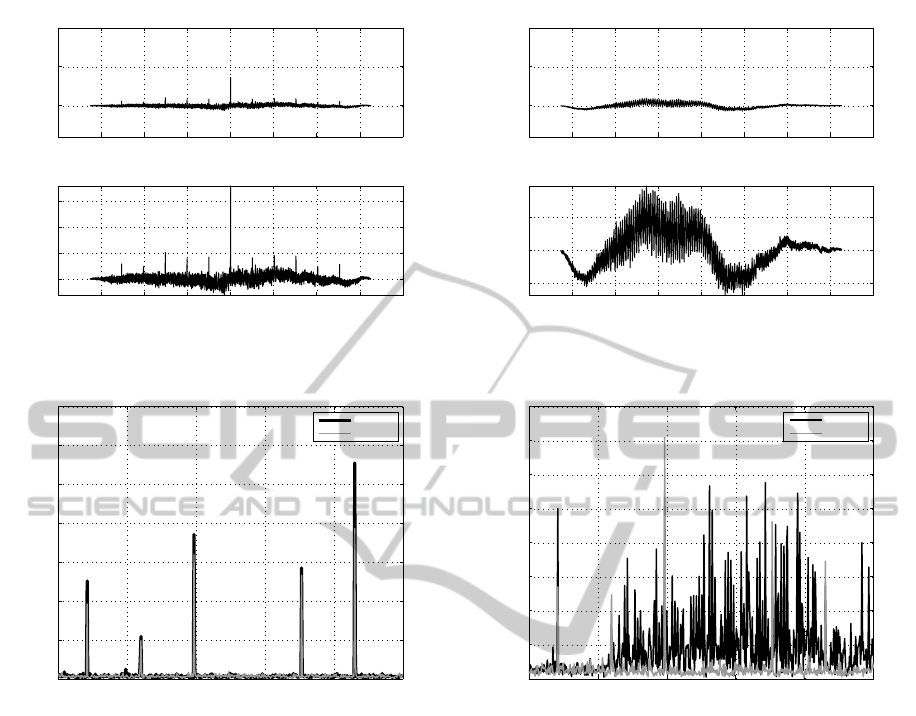
Figure 8: Channel 32, r
xy
(k) between nodes 0 and 1.
0 100 200 300 400 500
0
0.2
0.4
0.6
0.8
1
1.2
1.4
Fano factor over window of length 65
Window number
D
Node 01
Node 00
Figure 9: Channel 32, D for nodes 0 and 1.
in Fig. 8 it is clear that the maximum sample cross-
correlation for the two nodes was found at lag 0, indi-
cating complete synchronization between the exam-
ined RSSI time series. In Fig. 9 the Fano factor for
nodes 0 and 1 in channel 32 is presented. It is evident
that the levels of dispersion in the two signals are sim-
ilar with the higher dispersion values occurring at the
spikes. Consequently, we can safely characterize the
observed channel behavior as being similar between
nodes 0 and 1.
Nevertheless, there exist numerous cases where
the maximum sample cross-correlation is low, even
though the nodes agree on the classification of the
channel. Such cases include aligned spikes that have
different amplitudes, or cases where the spikes are
preserved but the mean and variance of the segments
between spikes vary significantly. In such cases, if
we rely on the maximization of the sample cross-
correlation to determine if the time series lag is within
acceptable synchronization error, it is possible to find
the maximum cross-correlation at a lag outside the
−4 −3 −2 −1 0 1 2 3 4
x 10
4
0
0.5
1
k
r
xy
(k)
Sample Cross−Correlation Function for Positive and Negative Lags
−4 −3 −2 −1 0 1 2 3 4
x 10
4
−0.05
0
0.05
k
r
xy
(k)
Sample Cross−Correlation Function for Positive and Negative Lags
Figure 10: Channel 32, r
xy
(k) between nodes 9 and 15.
0 100 200 300 400 500
0
0.05
0.1
0.15
0.2
0.25
0.3
0.35
0.4
Fano factor over window of length 65
Window number
D
Node 15
Node 09
Figure 11: Channel 32, D for nodes 9 and 15.
acceptable lags. In channel 32 such behavior is en-
countered in pairs composed of the nodes 8, 12 and
15. Specifically, Fig. 10 presents the sample cross-
correlation function for channel 32, between nodes 9
and 15. The differences in the signal amplitudes make
synchronization impossible, resulting in the maxi-
mum sample cross-correlation value occurring at lag
-12729. It is also notable that the absolute maximum
sample cross-correlation value is 0.0971 significantly
lower than the one in the synchronized time series of
the same channel presented in Fig. 8, which reached
the value 0.3610. Such disagreement is an indica-
tor that, at a microscopic level, the nodes observe
the channel as being drastically different despite their
consensus characterization as being of the same class.
Additionally, observing the Fano factor for nodes
9 and 15 in Fig. 11, we notice that the dispersion of
the received signal in node 15 is significantly different
and higher than the one in node 9, due to fluctuations
of the mean value. It is interesting to observe that
the large dispersion values for node 9, correspond to
AStudyofChannelClassificationAgreementinUrbanWirelessSensorNetworkEnvironments
255
times where spikes occur and totally overlap with the
dispersion values of node 15. As a result, even with
the presence of the spikes in both series and despite
the spikes being aligned/synchronized, the interven-
ing quiet segments of the channel observed by node
15 exhibit severe fluctuations compared to node 9.
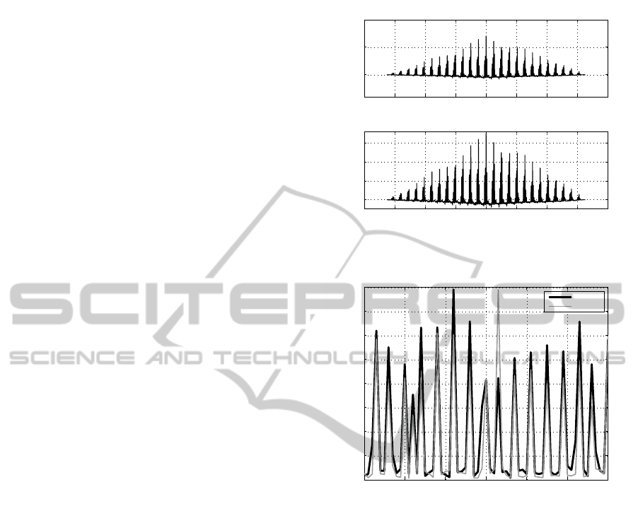
5.2 Quiet with Rapid Spikes (qrs)
Channel
Channel 61 represents the quiet with rapid spikes
pattern. High sample cross-correlation values were
encountered, as there are more synchronized spikes
to contribute to the sample cross-correlation statis-
tic. The interesting observation for this class is that
the (usually) periodic nature of the rapid spikes re-
sults in a sample cross-correlation which captures this
periodicity. Indeed, the peaks of the sample cross-
correlation occur at lags that are multiples of 250
with a variation between [−10, +10]. This behavior
is also captured in Fig. 12, which represents the sam-
ple cross-correlation between nodes 0 and 6. Observe
the high sample cross-correlation of 0.7242 for syn-
chronization at lag 0. Note that this behaviour is also
observed in other quiet with rapid spikes channels,
namely 58, 59, 63, and 81.
Furthermore, the Fano factor shown in Fig. 13
(zoomed into a range to clearly show the periodic na-
ture), reveals that for nodes 0 and 6 on channel 61, the
high dispersion values are present whenever a spike
occurs. Note that the Fano factor values are roughly
equal, suggesting similar mean and variance, confirm-
ing a very strong similarity on how the channel is ob-
served by the two nodes across the length of the trace.
5.3 Shifting Mean (sm) Channel
Channel 126 is an example of a shifting mean chan-
nel. Shifting mean channels were characterized
by overall higher maximum sample cross-correlation
values, frequently exceeding 0.9 and approaching 1.0.
For channel 126 the lag values were always accept-
able (within ±10). As an example, the maximum
sample cross-correlation value for the node pair 12
and 14 reaches the value 0.9827 at lag 0, as shown in
Fig. 14.
Nevertheless, there exists a notable exception, that
of pairs involving node 10, whose maximum sam-
ple cross-correlation values are somewhat lower in
the 0.30-0.70 region. The pair consisting of nodes
0 and 10 falls in this category and its sample cross-
correlation function is pictured in Fig. 7. In the ex-
amined case the maximum sample cross-correlation
−4 −3 −2 −1 0 1 2 3 4
x 10
4
0
0.5
1
k
r
xy
(k)
Sample Cross−Correlation Function for Positive and Negative Lags
−4 −3 −2 −1 0 1 2 3 4
x 10
4
0
0.2
0.4
0.6
k
r
xy
(k)
Sample Cross−Correlation Function for Positive and Negative Lags
Figure 12: Channel 61, r
xy
(k) between nodes 0 and 6.
180 190 200 210 220 230 240
0
0.05
0.1
0.15
0.2
0.25
0.3
0.35
0.4
Fano factor over window of length 65
Window number
D
Node 06
Node 00
Figure 13: Channel 61, D for nodes 0 and 6.
value is 0.6158 for lag 0, indicating absolute synchro-
nization. After a closer observation, we conclude that
even if the time series are near perfectly synchronized
(i.e., the level shifts occur at lag 0 or at most ±1 in
the two signals), the sample cross-correlation value
strongly depends on the levels of the mean and vari-
ance. Since the mean and variance are not necessarily
the same, low sample cross-correlation could be cal-
culated as a result.
5.4 Quiet (q) Channel
Channel 250 is an example of a quiet channel. Quiet
channels do not present any distinguishing charac-
teristics, like spikes. However, even if the variance
between a pair of quiet signals tends to stay at the
same levels, their mean values are not necessarily
similar. As a result, for quiet channels the sample
cross-correlation produces the lowest maximum val-
ues. These small maximum values can be as low as
in the 0.0 to 0.1 range. They rarely exceed 0.5. The
SENSORNETS2014-InternationalConferenceonSensorNetworks
256
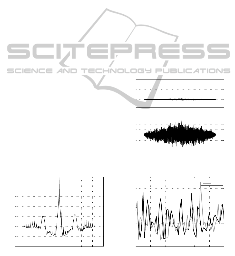
sample cross-correlation function of channel 250 be-
tween nodes 6 and 13 shown in Fig. 15, exhibits the
‘difficulty’ of the two signals to be synchronized. The
sample cross-correlation stays at extremely low levels
throughout the lags, while the maximum value 0.0552
is calculated for lag -159.
In Fig. 16 (zoomed into a range to clearly show
the lack of agreement), the cause becomes clearer as
the Fano factor values are totally disparate. This is
an indication of different mean values and variance.
As a result the synchronization of the time series be-
comes harder and, consequently, the sample cross-
correlation values remain in very low levels. In addi-
tion to channel 250, channels 212, 213, 214 and 215
exhibit the same behavior.
5.5 High and Level (hl) Channel
Channels characterized as high and level like 95, 160
and 225 present a behaviour similar to quiet channels.
High and level channels can also be characterized as
quiet but with higher amplitudes. Consequently, they
also follow the behaviour described in Section 5.4.
5.6 Aggregate Analysis of Node Pairs
We first analyze all pairs of nodes across all chan-
nels. 120 unique node pairs can be defined, which
multiplied by 256 channels give us 30720 pairs un-
der examination. Of those, 23438 node pairs agree
on the class to which they have classified the channel
and the remaining 7282 disagree on the class. Of the
23438 that agree on the class, 9696 exhibit maximum
sample cross-correlation at small lags ∈ [−10,10] that
indicate synchronization and correct classification of
the signals.
−4 −3 −2 −1 0 1 2 3 4
x 10
4
−0.4
−0.2
0
0.2
0.4
0.6
0.8
1
k
r
xy
(k)
Sample Cross−Correlation Function for Positive and Negative Lags
Figure 14: Channel 126, r
xy
(k) between nodes 12 and 14.
We first use this group of 9696 pairs for our con-
clusions on the linkage between cross-correlation and
classification, as shown in Table 1. It can be seen that
the quiet with rapid spikes and shifting mean chan-
nels class characterizations can be trusted as depict-
ing accurately the same channel state. The high and
level classification is debatable as a non-trivial per-
centage (42.9%) corresponds to low maximum cross-
correlation, which could indicate lack of actual cor-
relation, but still more than 50% exhibit significant
correlation. The quiet and the quiet with spikes classi-
fications are the most problematic because of the very
low cross-correlation.
Next, we illustrate the situation of complete con-
sensus, i.e., cases where we consider only the pairs
of nodes for channels in which all nodes have agreed
that the channel belongs to the same class. We pro-
vide Table 2. Note that consensus occurred in only
65 channels (q: 20, qs: 19, qrs: 12, hl: 5, sm: 9) but
the results are very similar to those when considering
−4 −3 −2 −1 0 1 2 3 4
x 10
4
0
0.5
1
k
r
xy
(k)
Sample Cross−Correlation Function for Positive and Negative Lags
−4 −3 −2 −1 0 1 2 3 4
x 10
4
−0.04
−0.02
0
0.02
0.04
k
r
xy
(k)
Sample Cross−Correlation Function for Positive and Negative Lags
Figure 15: Channel 250, r
xy
(k) between nodes 6 and 13.
180 190 200 210 220 230 240
0
0.005
0.01
0.015
0.02
0.025
0.03
Fano factor over window of length 65
Window number
D
Node 13
Node 06
Figure 16: Channel 250, D for nodes 6 and 13.
AStudyofChannelClassificationAgreementinUrbanWirelessSensorNetworkEnvironments
257

agreement of pairs of nodes across all channels (Ta-
ble 1), and therefore our observations stand the same.
Table 1: Percentages of the maximum r
xy
(k) occurring
at lags ∈ [−10,10] and with value falling within specific
bounds, for same-class node pairs.
max r
xy
(k) q qs qrs sm hl
[0,0.2) 48.0% 50.2% 1.7% 0.5% 42.9%
[0.2,0.4) 27.3% 39.0% 26.8% 2.7% 14.3%
[0.4,0.6) 16.1% 9.8% 47.9% 8.6% 28.6%
[0.6,0.8) 7.7% 0.9% 22.9% 13.5% 14.2%
[0.8,1) 0.9% 0.1% 0.7% 74.7% 0.0%
Table 2: Percentages of the maximum r
xy
(k) occurring
at lags ∈ [−10,10] and with value falling within specific
bounds, for channels where all nodes agree on the class.
max r
xy
(k) q qs qrs sm hl
[0,0.2) 63.1% 42.4% 0.5% 0.0% 42.9%
[0.2,0.4) 24.2% 45.5% 20.3% 0.8% 14.3%
[0.4,0.6) 6.0% 11.4% 48.5% 8.2% 28.6%
[0.6,0.8) 6.0% 0.6% 29.7% 13.6% 14.2%
[0.8,1) 0.7% 0.1% 1.0% 77.4% 0.0%
Table 3: Percentages of the maximum r
xy
(k) falling within
specific bounds for pairs of nodes that do not belong to the
same class.
max r
xy
(k) Percentage
[0,0.2) 66.0%
[0.2,0.4) 22.1%
[0.4,0.6) 7.9%
[0.6,0.8) 3.0%
[0.8,1) 0.1%
Table 4: Percentages of the maximum r
xy
(k) occurring at
lags ∈ [−35000,−10) or lags∈ (10,35000] and with value
falling within specific bounds, for same-class node pairs.
max r
xy
(k) q qs qrs sm hl
[0,0.2) 88.7% 81.9% 20.0% 4.0% 80.5%
[0.2,0.4) 9.4% 14.8% 54.5% 31.8% 14.0%
[0.4,0.6) 1.6% 2.9% 23.3% 21.6% 4.3%
[0.6,0.8) 0.2% 0.4% 2.2% 16.2% 0.9%
[0.8,1) 0.1% 0.0% 0.0% 26.4% 0.3%
Table 5: Percentages of the maximum r
xy
(k) occurring at
lags ∈ [−35000,−10) or lags∈ (10,35000] and with value
falling within specific bounds, for channels where all nodes
agree on the class.
max r
xy
(k) q qs qrs sm hl
[0,0.2) 94.8% 75.1% 13.3% 0.9% 85.2%
[0.2,0.4) 4.6% 20.2% 52.5% 23.6% 9.7%
[0.4,0.6) 0.5% 4.3% 30.4% 23.6% 4.0%
[0.6,0.8) 0.1% 0.4% 3.8% 19.8% 0.8%
[0.8,1) 0.0% 0.0% 0.0% 32.1% 0.3%
For the sake of comparison, we considered pairs
of nodes that disagreed on the channel class. This
is shown in Table 3 and confirms that the results for
quiet and quiet with spikes are readily comparable to
the case where the nodes observe what they classify
as completely different channel behaviors.
Finally, we consider the results for pairs (13742
of them) that were found to be “out–of–sync” with
respect to the lags. Clearly, this is a limitation of our
technique to synchronize the time series, but it can be
used to point out how a simple cross-correlation met-
ric is limiting the study of similarity between time se-
ries. As shown in Table 4 in the case of quiet with
rapid spikes, using the maximum cross–correlation
may result in favouring a large lag, primarily because
the amplitude of the periodic peaks further away in
time could be larger and add up to a numerically
higher cross-correlation at unnaturally large lags. We
conjecture that the same happens with the shifting
mean class because a pattern of shifts could be re-
peated at higher amplitude further away in the time
series than lag zero. Similar behavior is observed
when the dataset is limited to channels where all
nodes agree on the class, as shown in Table 5.
6 CONCLUSIONS
We have studied whether the cross-correlation be-
tween RSSI measurements carried out by WSN nodes
in the same network reflects accurately the consensus
about the channel state, had the nodes independently
decided on the channel state based on a classification
scheme. The results paint a mixed picture whereby
a consensus towards a shifting mean or a quiet with
rapid spikes classification can be trusted. However,
patterns that do not exhibit much dynamic behav-
ior, i.e., quiet, or high and level, or even quiet with
occasional spikes, are not characterized by a cross-
correlation much higher than what would have been
if there was no agreement on the class of the traces
at all. The recommendation therefore is that, if con-
sensus algorithms are to be utilized, a very reliable
per-node classifier for quiet, high and level, or quiet
with spikes channel would be necessary.
Our study is far from perfect. For example, the use
of cross-correlation as the means of studying similar-
ity between time series over their entire length does
not reveal possible short-term similarities that do not
necessarily persist or are, numerically speaking, di-
luted over a long time period. We are therefore con-
sidering extensions that allow the extraction of short-
term and long-term similarities. Additionally, we are
well aware that more information could be used to an-
notate the classification, i.e., the period for periodic
spikes. Nevertheless, we point out that a (summa-
SENSORNETS2014-InternationalConferenceonSensorNetworks
258

rized) description based on temporal characteristics
that further “parameterize” the class would also need
some common synchronization adjustment, this time
performed in real-time during the RSSI data collec-
tion. In short, the classification becomes a combined
classification and parameter estimation problem.
ACKNOWLEDGEMENTS
The authors would like to thank Dr. Nicholas Boers
and OlsoNet Communications Corp. for their tech-
nical support. This work has been partially funded
by the Natural Sciences and Engineering Research
Council of Canada (NSERC).
REFERENCES
Akhmetshina, E., Gburzynski, P., and Vizeacoumar, F.
(2003). Picos: A tiny operating system for extremely
small embedded platforms. In Las Vegas, pages 116–
122.
Akyildiz, I. F., Lo, B. F., and Balakrishnan, R. (2011).
Cooperative spectrum sensing in cognitive radio net-
works: A survey. Phys. Commun., 4(1):40–62.
Boers, N., Chodos, D., Huang, J., Gburzynski, P., Niko-
laidis, I., and Stroulia, E. (2009). The smart condo:
visualizing independent living environments in a vir-
tual world. In Pervasive Computing Technologies for
Healthcare, 2009. PervasiveHealth 2009. 3rd Interna-
tional Conference on, pages 1–8.
Boers, N., Nikolaidis, I., and Gburzynski, P. (2010). Pat-
terns in the rssi traces from an indoor urban environ-
ment. In Computer Aided Modeling, Analysis and
Design of Communication Links and Networks (CA-
MAD), 2010 15th IEEE International Workshop on,
pages 61–65.
Boers, N. M., Nikolaidis, I., and Gburzynski, P. (2012a).
Impulsive interference avoidance in dense wireless
sensor networks. In Proceedings of the 11th inter-
national conference on Ad-hoc, Mobile, and Wireless
Networks, ADHOC-NOW’12, pages 167–180, Berlin,
Heidelberg. Springer-Verlag.
Boers, N. M., Nikolaidis, I., and Gburzynski, P. (2012b).
Sampling and classifying interference patterns in a
wireless sensor network. ACM Trans. Sen. Netw.,
9(1):2:1–2:19.
Bourke, P. (1996). Cross correla-
tion,autocorrelation , 2d pattern identification.
http://paulbourke.net/miscellaneous/correlate/. [On-
line; accessed 2013].
Lee, H., Cerpa, A., and Levis, P. (2007). Improving wireless
simulation through noise modeling. In Proceedings of
the 6th international conference on Information pro-
cessing in sensor networks, IPSN ’07, pages 21–30,
New York, NY, USA. ACM.
Olsonet (2008). Platform for rd in sensor networking.
http://www.olsonet.com/Documents/emspcc11.pdf.
[Online; accessed 2013].
AStudyofChannelClassificationAgreementinUrbanWirelessSensorNetworkEnvironments
259
