Training Optimum-Path Forest on Graphics Processing Units

Adriana S. Iwashita

, Marcos V. T. Romero

, Alexandro Baldassin

, Kelton A. P. Costa

and Jo

ao P. Papa

Department of Computing, S

ao Paulo State University, Bauru, S

ao Paulo, Brazil

Department of Statistics, Applied Mathematics and Computation, S

ao Paulo State University, Rio Claro, S

ao Paulo, Brazil

Keywords:

Optimum-Path Forest, Graphics Processing Unit.

Abstract:

In this paper, we presented a Graphics Processing Unit (GPU)-based training algorithm for Optimum-Path

Forest (OPF) classiﬁer. The proposed approach employs the idea of a vector-matrix multiplication to speed

up both traditional OPF training algorithm and a recently proposed Central Processing Unit (CPU)-based

OPF training algorithm. Experiments in several public datasets have showed the efﬁciency of the proposed

approach, which demonstrated to be up to 14 times faster for some datasets. To the best of our knowledge, this

is the ﬁrst GPU-based implementation for OPF training algorithm.

1 INTRODUCTION

Pattern recognition techniques have as the main goal

to learn a discriminative function that separates the

dataset samples in different classes. Such learning

process is performed over a training set, which can

be labeled or not, and the effectiveness of the classi-

ﬁer is assessed on a testing set (Duda et al., 2000).

Thus, the learning is the most important phase of a

classiﬁer, and also the most computational expensive.

In the recent years, there is a considerable number

of works that focuses on developing machine learn-

ing algorithms on Graphics Processing Units (GPUs).

Catanzaro et al. (Catanzaro et al., 2008), for instance,

presented a GPU-based implementation for the well-

known Support Vector Machines (SVM) classiﬁer,

which was about 9 − 35× faster when compared to

the traditional CPU (Central Processing Unit) imple-

mentation.

In the same year, Do et al. (Do et al., 2008) also

proposed an SVM implementation on GPUs, and Jang

et al. (Jang et al., 2008) presented an Artiﬁcial Neu-

ral Network (ANN) version using Compute Uniﬁed

Device Architecture (CUDA) and OpenMP (Open

Multi-Processing), which is a library for concurrent

programming. In this work, the authors highlighted

the importance of considering the real needs of mas-

sive programming, i.e., the algorithms that will be im-

plemented in such parallel environments need to con-

tain modules that can be executed concurrently. Oth-

erwise, the throughput of data interchange between

processors may degrade the performance of the whole

system.

Papa et al. (Papa et al., 2009a; Papa et al., 2012)

proposed a pattern recognition technique called Opti-

mum Path Forest (OPF) aiming to overcome the time

spent with the learning phase. They showed that OPF

can obtain similar effectiveness to SVM, but it can be

faster in the training phase. The OPF models the prob-

lem of pattern recognition as a graph partition into

optimum-path trees (OPTs), which are rooted by key

samples (prototypes) that compete among themselves

in order to conquer the remaining samples. Further,

Iwashita et al. (Iwashita et al., 2012) proposed an opti-

mization of the OPF training algorithm in CPU, being

such approach up to two times faster than traditional

OPF with similar recognition rates.

In this paper, we presented an GPU-based imple-

mentation of the OPF training phase, which can be

faster than traditional OPF and also more efﬁcient

than the approach proposed in (Iwashita et al., 2012).

We have validated the proposed technique using sev-

eral public datasets. As far as we know, this is the ﬁrst

GPU-based implementation of the OPF classiﬁer. The

remainder of this paper is organized as follows. Sec-

tions 2 and 3 present the OPF background and the pro-

posed CUDA-based training algorithm, respectively.

Section 4 discusses the experimental results, and Sec-

tion 5 states conclusions.

581

S. Iwashita A., V. T. Romero M., Baldassin A., A. P. Costa K. and P. Papa J..

Training Optimum-Path Forest on Graphics Processing Units.

DOI: 10.5220/0004737805810588

In Proceedings of the 9th International Conference on Computer Vision Theory and Applications (VISAPP-2014), pages 581-588

ISBN: 978-989-758-004-8

 2014 SCITEPRESS (Science and Technology Publications, Lda.)

2 PATTERN CLASSIFICATION

USING OPTIMUM-PATH

FOREST

Let Z = Z

∪ Z

be a dataset were Z

and Z

are the

training and test sets, respectively, with |Z

| and |Z

samples. Let λ(s) be the function which associates the

correct label i, i = 1,2,. . . , c to any sample s ∈ Z

∪Z

from class i. Let S ∈ Z

be the set of prototype sam-

ples, and let ~v be the algorithm that extracts n features

from any sample s ∈ Z

∪Z

, and return a feature vec-

tor ~v(s) ∈ ℜ

. The distance d(s,t) between two sam-

ples, s and t, is given by the distance between his fea-

ture vectors ~v(s) e ~v(t). The problem consists in use

S, (~v,d), Z

and Z

to project an optimal classiﬁer,

which can predict the correct label λ(s) of any sample

s ∈ Z

Let (Z

,A) be a complete graph in which nodes

are samples in Z

, where any pair of samples deﬁnes

a edge on A (i.e., A = Z

), creating a completed

weighted graph of Z

set. A path is a sequence of

samples π =

,. . . , s

, where (s

i+1

) ∈ A for

1 ≤ i ≤ k − 1. A path is said to be trivial if π = hs

It is associated for each path π the cost given by a

smooth cost function f (Falc

ao et al., 2004), denoted

by f (π). A path is optimum if f (π) ≤ f (τ) for any

path τ, where π and τ ends in the same sample s, re-

gardless of their origin. We also denote π · hs,ti the

concatenation of the path π ending in s and edge (s,t).

The OPF algorithm can be used with any soft cost

function, which can combine samples with similar

properties (Falc

ao et al., 2004). However, the OPF

was designed using the f

max

cost function, due to

its theoretical properties to estimate optimum proto-

types (All

ene et al., 2007):

max

(hsi) =



0 if s ∈ S,

+∞ otherwise

max

(π · hs,ti) = max{ f

max

(π),d(s,t)}, (1)

the f

max

(π) compute the maximum distance between

adjacent samples in π, when π is not a trivial path.

The OPF algorithm associates an optimal path

∗

(s) of S to all samples s ∈ Z

, making a optimum

path forest P (a function without cycles which asso-

ciates to all s ∈ Z

his predecessor P(s) in P

∗

(s), or

assigns nil when s ∈ S). Let R(s) ∈ S the root of

∗

(s) which can be achieved using P(s). The OPF

algorithm computes, for each s ∈ Z

, the cost V(s) of

∗

(s), the label L(s) = λ(R(s)) and his predecessor

P(s).

We say S

∗

is an optimum set of prototypes when

the algorithm propagates the labels L(s) = λ(s) for all

s ∈ Z

. Thus, S

∗

can be found by exploring the the-

oretical relationship between the Minimum Spanning

Tree (MST) (All

ene et al., 2007) and the minimum

path tree to f

max

. The training consists essentially of

two steps: ﬁnding S

∗

and a OPF classiﬁer rooted at

∗

When we compute a MST on the completed graph

,A), we obtain a connected acyclic graph whose

nodes are all the samples in Z

, and the edges are not

directed and weighted. Their weights are given by the

distance d between the features vectors of adjacent

samples. This spanning tree is optimum in the sense

that the sum of the weights of its edges is minimal

compared to other spanning trees on the completed

graph. On MST, each pair of samples is connected by

a path, which is optimum under f

max

The optimum prototypes are the connected ele-

ments on MST with different labels Z

, i.e., the clos-

est elements from different classes. By removing the

edges between different classes, such adjacent sam-

ples become prototypes in S

∗

and can compute an

optimum path forest without misclassiﬁcation at Z

(competition process). Therefore, each prototype de-

ﬁnes its own Optimum-Path Tree (OPT), and the col-

lection of all OPT’s deﬁne the optimum-path forest,

which gives the name to the classiﬁer.

The classiﬁcation step is straightforward, i.e.,

given a test sample s ∈ Z

, we connect it to all train-

ing nodes of the optimum-path forest generated in the

training phase, and we evaluate which node p ∈ Z

minimizes the equation below:

V (s) = min

∀Z

max{V (p),d(p,s)}. (2)

Thus, the node p ∈ Z

that minimizes V (s) will be the

one that conquer s.

3 TRAINING OPTIMUM-PATH

FOREST ON CUDA

The implementation of the OPF training phase on

CUDA environment was conducted using particular

code instructions to execute similar actions in paral-

lel. As graphics cards have their processing structures

organized into parallel architectures, it is important to

shed light over the implemented algorithms must have

parallelizable modules to obtain performance gain.

As described in Section 2, the OPF training step

is composed by two modules: (i) the ﬁrst one com-

putes the MST over the complete graph and marks

the connected elements with different labels as proto-

types; and (ii) with prototypes in hand, we can pro-

ceed with the competition process between them to

build the OPTs.

The proposed GPU-based implementation of OPF

VISAPP2014-InternationalConferenceonComputerVisionTheoryandApplications

582

classiﬁer also employs the above idea, i.e., we ﬁrst

paralleled the MST computation and then the com-

petition process between prototypes. For both ap-

proaches, there are three main steps: to ﬁnd the el-

ement p with lowest cost that will try to conquer the

other nodes, to calculate the distance between node p

and other nodes, and to verify whether the node p can

conquer other nodes or not.

In this paper, we adopted a similar procedure to

compute the MST and the optimum-path forest. The

methodology is basically the same, i.e., one needs to

ﬁnd the node with lowest cost to begin the competi-

tion process. Considering the MST computation, for

instance, the root node r will be associated with cost

0, and the remaining nodes with cost +∞. Thus, we

can force r to control the MST computation. The next

step is to compute the distance between r and the re-

maining nodes to ﬁnd out the shortest one, which will

be the new leader, i.e., the sample t with lowest cost.

This procedure can be conducted using f

sum

, which is

similar to f

max

path-cost function (Equation 1):

sum

(hsi) =



0 if s ∈ S,

+∞ otherwise

sum

(π · hs,ti) = f

sum

(π) + d(s,t). (3)

In this case, S stands for the set of root nodes. In

the context of MST computation, we have only one

root node. As one can see, the cost offered to t is just

the summation of the cost of s with the distance (arc-

weight) between s and t. Notice that we can slightly

change some points to make the above procedure ca-

pable to compute the optimum-pat forest: instead of

using just one node root to begin the competition al-

gorithm to compute MST, we can now use a set of

prototype nodes, i.e., the connected nodes in the min-

imum spanning tree with different labels. Then, we

can place f

max

instead of f

sum

and execute the compe-

tition process again.

In regard to the ﬁrst step, i.e., to ﬁnd out the ele-

ment with the lowest cost, we employed the primitive

min element from Thrust (Hoberock and Bell, 2010)

library, which returns the element with the lowest cost

from a set of nodes using parallel algorithms. Thrust

is a library to the development of parallel algorithms

based on the C++ STL (Standard Template Library),

and works like a high-level interface to increase de-

veloper productivity.

The next step is to compute the distance between

the current node and the remaining ones. In this case,

we employed a collection of threads to take care of a

set of nodes. This means the distance between node

p and the remaining nodes of the graph will be com-

puted in parallel using an approach similarly to a mul-

tiplication of a matrix by a vector (Fujimoto, 2008).

The rows of this matrix, called here as “feature ma-

trix” , are the training set nodes represented by their

feature vectors. This matrix is allocated in the tex-

ture memory, and can be accessed by all threads; the

feature vector of a node p is allocated on the global

memory.

A thread is allocated for each element of the fea-

ture matrix, which will calculate the distance between

an element of the matrix with node p, storing this re-

sult in a “partial results matrix”. Each block of threads

has an array of partial results, which are allocated in

the shared memory of them. The ﬁnal result (dis-

tances between p and other nodes) is a distance vec-

tor allocated on the global memory, in which posi-

tion i means the distance between nodes p and i. The

level of parallelism of these operations can be classi-

ﬁed as ﬁne-granularity, since there are a large number

of small and simple processes running on the instruc-

tion level.

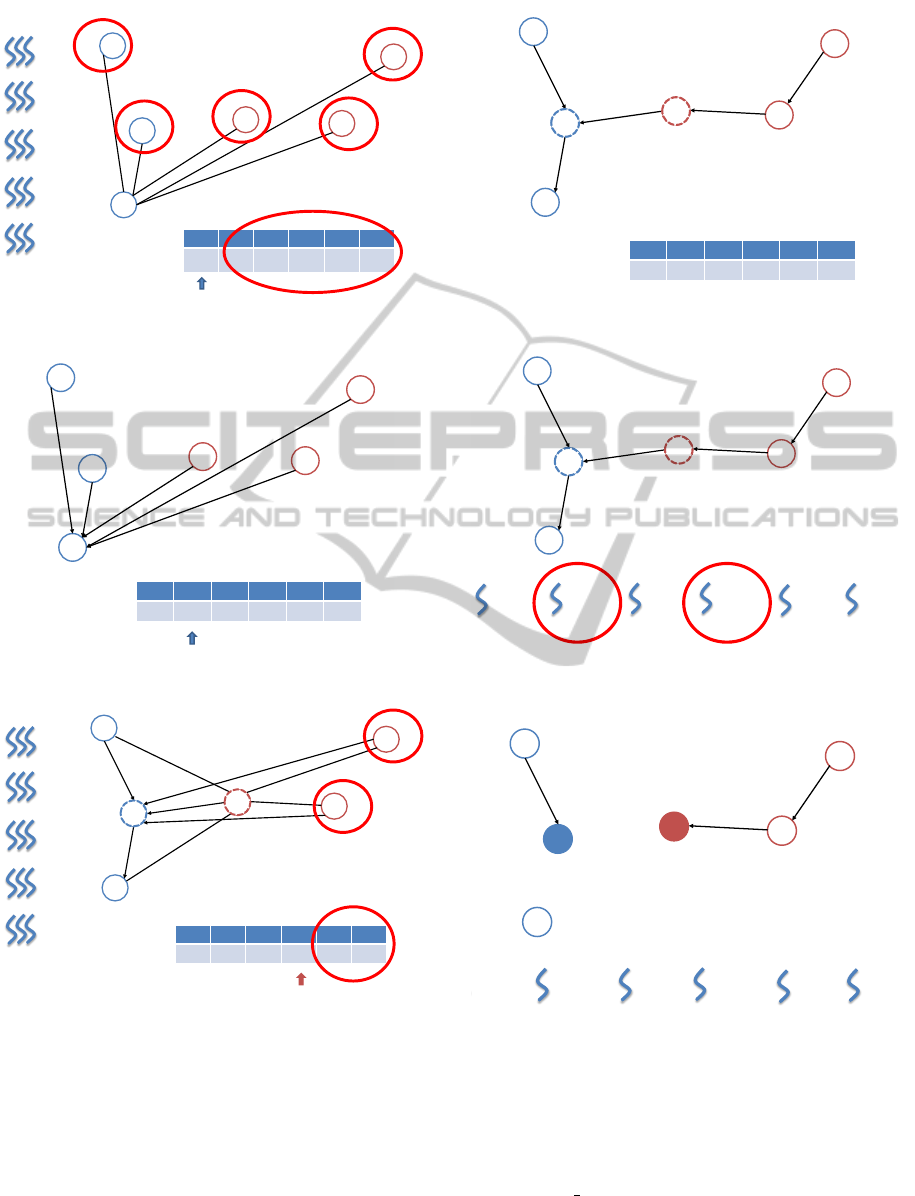
Figures 2 to 10 exempliﬁes the proposed ap-

proach. Figure 1 illustrates the training set: the graph

nodes are initialized with cost ∞, and the node 1 will

be the root of the MST; thus the cost 0 is assigned to

it. As aforementioned, the ﬁrst step of OPF training

algorithm is to compute the MST and to ﬁnd the pro-

totypes. In Figure 2, we can face the situation when

the proposed algorithm is in the ﬁrst iteration (MST

computation). Using the min element primitive, node

1 leaves the queue to conquer the remaining nodes,

since it has the lowest cost. The set of GPU threads is

responsible for calculating the distance between node

1 and the other nodes; it also veriﬁes whether the node

cost is lower than the distance offered by node 1.

Figure 3 illustrates the situation after the ﬁrst iter-

ation, and the selection of node 2 (using min element

primitive) as the next dominant node. The dotted

nodes in Figure 4 represent the prototypes found out

after the 4th iteration. The arrow highlights the node

4, which will begin the conquering process. As

showed in Figure 2, node 4 now leaves the queue to

conquer the other nodes, and the set of GPU threads is

Priority queue

∞

Figure 1: Training set.

TrainingOptimum-PathForestonGraphicsProcessingUnits

583

2.8

5.5

13.4

10.6

∞

d1 = 7

d2 = 2.8

d3 = 5.5

d4 = 13.4

d5 = 10.6

∞

Priority queue

Figure 2: First iteration of the MST algorithm.

2.8

5.5

10.6

13.4

2.8

5.5

10.6

13.4

Priority queue

Figure 3: Step 2 of the MST algorithm.

2.8

9.8

12.4

d1 = 5.5

d2 = 4

d3 = 6

d4 = 7

d5 = 3.8

2.8

9.8

12.4

3.8

5.5

Priority queue

Figure 4: After the 4th iteration, two prototypes are found

out and node 4 now conquers two nodes.

responsible for calculating the distance between node

4 and the other nodes.

Figure 5 depicts the ﬁnal MST, and the dotted

nodes stand for the prototypes. Figure 6 illustrates

the set of nodes after the MST construction. In this

phase, each thread is responsible for updating a node,

i.e., each thread veriﬁes whether the node has been as-

signed as a prototype or not. If the node is prototype,

the thread updates the node cost to 0 and updates this

2.8

3.8

2.6

2.8

3.8

2.6

Priority queue

Figure 5: MST generated for the training set.

2.8

3.8

2.6

p1 = 0

p2 = 1 p3 = 0 p4 = 1

p5 = 0

p6 = 0

Figure 6: Each thread responsible for checking whether a

node is a prototype or not.

∞

p1 = 0

p2 = 1 p3 = 0 p4 = 1

p5 = 0

p6 = 0

Figure 7: Each thread updates the cost of the node; and if it

is also a prototype, the thread updates its predecessor.

predecessor node to NIL. If the node is not a proto-

type, this cost value will be ∞. Figure 7 illustrates the

nodes after the aforementioned updating process.

Figure 8 illustrates the 2nd phase of the training

step: the min element primitive chooses the prototype

node 2 to leave the queue and then to conquer the re-

maining nodes.

Figure 9 shows the node 2 on action: each set

VISAPP2014-InternationalConferenceonComputerVisionTheoryandApplications

584

∞

Priority queue

Figure 8: Graph with the prototypes marked: 2nd phase of

the training step.

2.8

9.8

12.4

∞

d1 = 2.8

d2 = 3

d3 = 12.4

d4 = 4

d5 = 9.8

If Max{0; dist(2,n)} < w(n)

Priority queue

Figure 9: Each set of threads calculates the distance be-

tween 2 and the other nodes.

2.8

3.8

Figure 10: Resulting optimum-path forest.

of GPU threads is responsible for calculating the dis-

tance between node 2 and the other nodes. Using the

path-cost function f

max

(Equation 1), node 2 tries to

conquer the other nodes.

Finally, Figure 10 presents the resulting optimum-

path forest using the proposed algorithm.

4 EXPERIMENTS

In this section, we discuss the experiments conducted

in order to show the efﬁciency of the proposed opti-

mization for OPF training step. We have used several

public datasets with different sizes to assess the train-

ing efﬁciency, and also the classiﬁcation accuracy in

distinct scenarios. Table 1 presents the datasets used

in this work.

Table 1: Datasets used in the experiments. With respect to

Covtype, we have used 25% of the original dataset.

Dataset # Samples # Features

Connect (Frank and Asuncion, 2013) 67557 126

Indian Pine (Landgrebe, 2005) 21025 220

Letter (King et al., 1995) 15000 16

Mnist (LeCun et al., 1988) 60000 780

Poker (Frank and Asuncion, 2013) 25010 10

Salinas (Kaewpijit et al., 2003) 111104 204

In regard to training and test set sizes, we em-

ployed a cross-validation procedure with different

percentages for that sets, which range from 10% to

90% of the training set size, with steps of 10. In or-

der to validate the proposed GPU-based OPF train-

ing algorithm, we have compared it against traditional

OPF and the optimization presented by Iwashita et

al. (Iwashita et al., 2012).

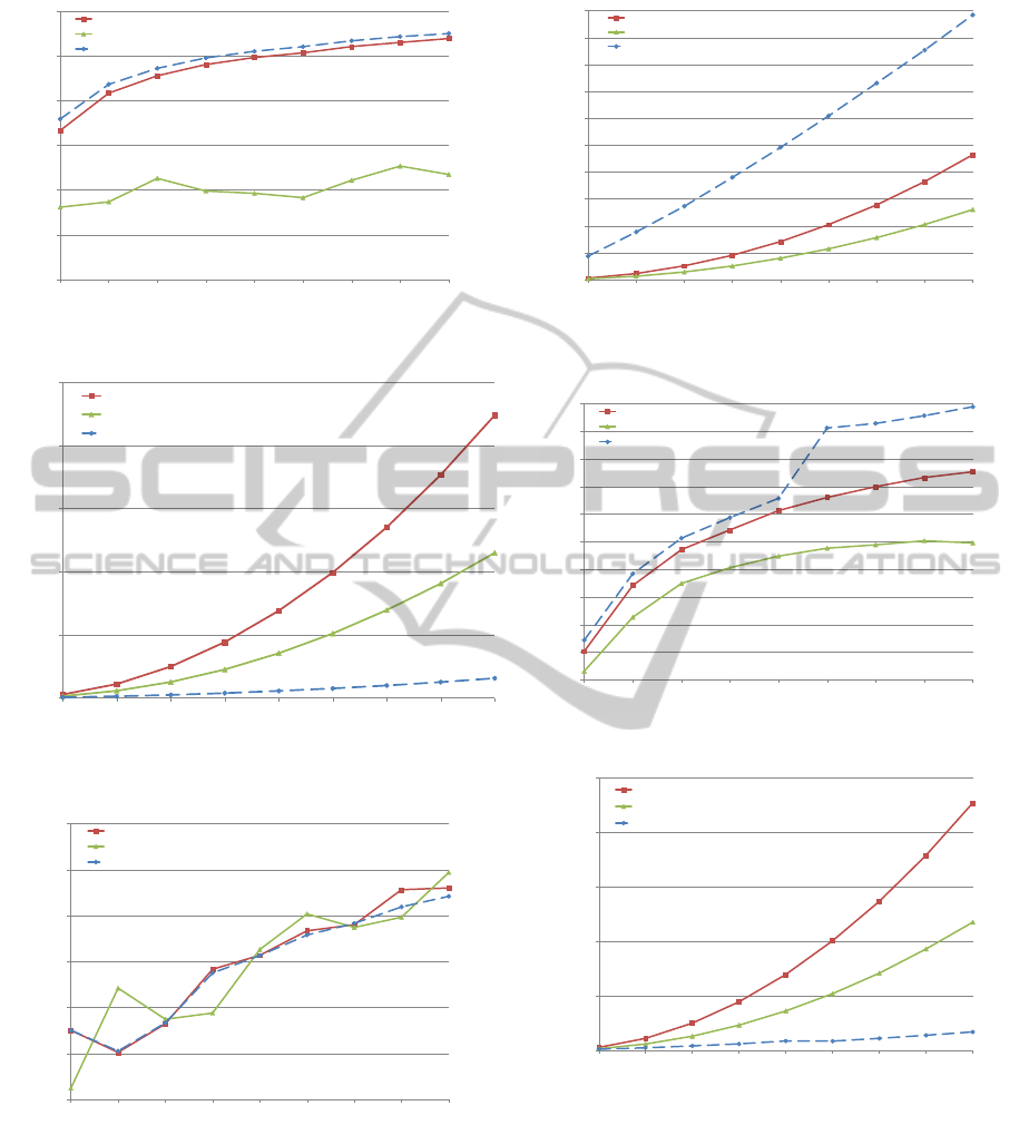
Figures 11 and 12 display, respectively, the mean

accuracy and training times with different percentages

of training and test sets for Connect dataset. Notice

the proposed approach has a gain about 2.523 with

30% of the training set. If we consider 90% of train-

ing dataset, the GPU-based OPF is about 5.522 faster

than traditional one. Notice the accuracies are also

similar among the compared techniques, being the

proposed approach also faster than the algorithm pro-

posed by (Iwashita et al., 2012).

Figures 13 and 14 display, respectively, the mean

accuracy and training times for Indian Pine dataset.

Considering 40% of the training set size, the proposed

approach has been 2.004 times faster for training than

traditional OPF. If we take into account 90% of train-

ing set size, the gain of GPU-based OPF is 4.021

times when compared with traditional OPF.

Figures 15 and 16 display, respectively, the mean

accuracy and training times for Letter dataset. Notice

the proposed approach was 1.825 times slower than

traditional OPF with 90% of the training set size. This

same behaviour can be observed with Poker dataset

(Figures 19 and 20). The problem concerns with the

few number of features in these datasets, which did

not compensate the data interchange between CPU

and GPU, since the distances are also computed us-

ing different threads.

Figures 17 and 18 display, respectively, the mean

accuracy and training times for Mnist dataset. In this

TrainingOptimum-PathForestonGraphicsProcessingUnits

585

62,5

63,5

64,5

65,5

Traditional OPF

Optimization proposed by [2]

Cuda OPF

Training set percentage

Mean accuracy

[7]

Figure 11: Mean classiﬁcation accuracy for Connect

dataset.

100

150

200

250

300

350

400

450

Traditional OPF

Optimization proposed by [2]

Cuda OPF

Training set percentage

Mean execution time [s]

[7]

Figure 12: Mean execution times in seconds with respect to

training step for Connect dataset.

Traditional OPF

Optimization proposed by [2]

Cuda OPF

Training set percentage

Mean accuracy

[7]

Figure 13: Mean classiﬁcation accuracy for Indian Pine

dataset.

case, we can see a gain of 14.405 times with 90%

of the training size of the proposed approach when

compared against with traditional OPF.

Figures 21 and 22 display, respectively, the mean

accuracy and training times for Salinas dataset. If we

consider 10% of the training set size, the proposed

approach is 3.038 times faster than traditional OPF; if

we take into account 90% of the training set size, the

Traditional OPF

Optimization proposed by [2]

Cuda OPF

Training set percentage

Mean execution time [s]

[7]

Figure 14: Mean execution times in seconds with respect to

the training step for Indian Pine dataset.

Traditional OPF

Optimization proposed by [2]

Cuda OPF

Training set percentage

Mean accuracy

[7]

Figure 15: Mean classiﬁcation accuracy for Letter dataset.

Traditional OPF

Optimization proposed by [2]

Cuda OPF

Training set percentage

Mean execution time [s]

[7]

Figure 16: Mean execution times in seconds with respect to

the training step for Letter dataset.

proposed approach is 13.580 faster than traditional

OPF. In this case, the GPU-based OPF has been more

accurate than the compared variants.

5 CONCLUSIONS

In this paper, we presented a GPU-based training al-

gorithm of the OPF classiﬁer. Our approach employs

VISAPP2014-InternationalConferenceonComputerVisionTheoryandApplications

586

Traditional OPF

Optimization proposed by [2]

Cuda OPF

Training set percentage

Mean accuracy

[7]

Figure 17: Mean classiﬁcation accuracy for Mnist dataset.

500

1000

1500

2000

2500

Traditional OPF

Optimization proposed by [2]

Cuda OPF

Training set percentage

Mean execution time [s]

[7]

Figure 18: Mean execution times in seconds with respect to

training step for Mnist dataset.

51,5

51,7

51,9

52,1

52,3

52,5

52,7

Traditional OPF

Optimization proposed by [2]

Cuda OPF

Training set percentage

Mean accuracy

[7]

Figure 19: Mean classiﬁcation accuracy for Poker dataset.

the idea of a vector-matrix parallel multiplication, in

which the same framework is employed for both MST

and optimum-path forest computation.

Experimental results have shown that the pro-

posed technique have obtained similar recognition

rates to those obtained by the traditional approach and

the CPU-based optimization proposed by Iwashita et

al. (Iwashita et al., 2012). Additionally, the proposed

Traditional OPF

Optimization proposed by [2]

Cuda OPF

Training set percentage

Mean execution time [s]

[7]

Figure 20: Mean execution times in seconds with respect to

the training step for Poker dataset.

Traditional OPF

Optimization proposed by [2]

Cuda OPF

Training set percentage

Mean accuracy

[7]

Figure 21: Mean classiﬁcation accuracy for Salinas dataset.

500

1000

1500

2000

2500

Traditional OPF

Optimization proposed by [2]

Cuda OPF

Training set percentage

Mean execution time [s]

[7]

Figure 22: Mean execution times in seconds with respect to

the training step for Salinas dataset.

approach has been faster for training, except when we

have datasets with a few features. In this case, the

throughput of the data interchange between CPUs and

GPUs did not compensate the parallelization effort. In

datasets with a considerable number of features, we

have observed a gain up to 14 times.

TrainingOptimum-PathForestonGraphicsProcessingUnits

587

ACKNOWLEDGEMENTS

The authors are grateful to FAPESP grants #2009/

16206-1, #2010/12697-8 and #2011/08348-0, and

CNPq grants #470571/2013-6 and #303182/2011-3.

REFERENCES

All

ene, C., Audibert, J. Y., Couprie, M., Cousty, J., and

Keriven, R. (2007). Some links between min-cuts,

optimal spanning forests and watersheds. In Proceed-

ings of the International Symposium on Mathematical

Morphology, pages 253–264. MCT/INPE.

Catanzaro, B., Sundaram, N., and Keutzer, K. (2008). Fast

support vector machine training and classiﬁcation on

graphics processors. In Proceedings of the 25th inter-

national conference on Machine learning, pages 104–

111, New York, NY, USA. ACM.

Do, T.-N., Nguyen, V.-H., and Poulet, F. (2008). Speed

up svm algorithm for massive classiﬁcation tasks. In

Proceedings of the 4th international conference on

Advanced Data Mining and Applications, pages 147–

157, Berlin, Heidelberg. Springer-Verlag.

Duda, R. O., Hart, P. E., and Stork, D. G. (2000). Pattern

Classiﬁcation (2nd Edition). Wiley-Interscience.

Falc

ao, A., Stolﬁ, J., and Lotufo, R. (2004). The image

foresting transform theory, algorithms, and applica-

tions. IEEE Transactions on Pattern Analysis and Ma-

chine Intelligence, 26(1):19–29.

Frank, A. and Asuncion, A. (2013). UCI machine learning

repository.

Fujimoto, N. (2008). Faster matrix-vector multiplication on

geforce 8800gtx. In Proceedings of the IEEE Inter-

national Symposium on Parallel and Distributed Pro-

cessing, pages 1–8.

Hoberock, J. and Bell, N. (2010). Thrust: A

Parallel Template Library. Available at

http://www.meganewtons.com/, Version 1.3.0.

Iwashita, A. S., Papa, J. P., Falc

ao, A. X., Lotufo, R.,

Oliveira, V. M., Albuquerque, V. H. C., and Tavares,

J. M. R. S. (2012). Speeding up optimum-path forest

training by path-cost propagation. In Proceedings of

the XXI International Conference on Pattern Recogni-

tion, pages 1233–1236.

Jang, H., Park, A., and Jung, K. (2008). Neural network im-

plementation using cuda and openmp. In DICTA ’08:

Proceedings of the 2008 Digital Image Computing:

Techniques and Applications, pages 155–161, Wash-

ington, DC, USA. IEEE Computer Society.

Kaewpijit, S., Moigne, J., and El-Ghazawi, T. (2003).

Automatic reduction of hyperspectral imagery using

wavelet spectral analysis. IEEE Transactions on Geo-

science and Remote Sensing, 41(4):863–871.

King, R. D., Feng, C., and Sutherland, A. (1995). Stat-

log: Comparison of classiﬁcation algorithms on large

real-world problems. Applied Artiﬁcial Intelligence,

9(3):289–333.

Landgrebe, D. (2005). Signal Theory Methods in Multi-

spectral Remote Sensing. Wiley, Newark, NJ.

LeCun, Y., Bottou, L., Bengio, Y., and Haffner, P. (1988).

Gradient-based learning applied to document recogni-

tion. Available at http://yann.lecun.com/exdb/mnist/.

Papa, J. P., Falc

ao, A. X., Albuquerque, V. H. C., and

Tavares, J. M. R. S. (2012). Efﬁcient supervised

optimum-path forest classiﬁcation for large datasets.

Pattern Recognition, 45(1):512–520.

Papa, J. P., Falc

ao, A. X., and Suzuki, C. T. N. (2009a).

Supervised pattern classiﬁcation based on optimum-

path forest. International Journal of Imaging Systems

and Technology, 19(2):120–131.

Papa, J. P., S., C. T. N., and Falc

ao, A. X. (2009b).

LibOPF: A library for the design of optimum-path

forest classiﬁers. Software version 2.0 available at

http://www.ic.unicamp.br/ afalcao/LibOPF.

VISAPP2014-InternationalConferenceonComputerVisionTheoryandApplications

588