Structure from Motion

ToF-aided 3D Reconstruction of Isometric Surfaces

S. Jafar Hosseini and Helder Araujo

Institute of Systems and Robotics, Department of Electrical and Computer Engineering,

University of Coimbra, Coimbra, Portugal

Keywords:

Structure from Motion, Isometric Surface, ToF Camera, 3D Reconstruction.

Abstract:

This paper deals with structure-from-motion (SfM) for non-rigid surfaces that undergo isometric motion. Our

SfM framework aims at the joint estimation of the 3D surface and the camera motion by combining a ToF

range sensor and a monocular RGB camera through a template-based approach. Our goal is to use the 2D

low-resolution depth estimates provided by the TOF camera, in order to facilitate the estimation of non-rigid

structure using the high-resolution images obtained by means of a RGB camera. In this paper, we model

isometric surfaces with a triangular mesh. The ToF sensor is used to obtain the depth of a sparse set of 3D

feature points, from which the depth of the mesh vertices can be recovered using a multivariate linear system.

Subsequently, we form a non-linear constraint based on the projected length of each edge. A second non-linear

constraint is then used for minimizing re-projection errors. These constraints are ﬁnally incorporated into an

optimization scheme to solve for structure and motion. Experimental results show that the proposed approach

has good performance even if only a low-resolution depth image is used.

1 INTRODUCTION

Structure-from-motion can be deﬁned as the problem

of simultaneous inference of the motion of a cam-

era and the 3D geometry of the scene solely from a

sequence of images. SfM was also extended to the

case of deformable objects. Non-rigid SfM is under-

constrained, which means that the recovery of non-

rigid 3D shape is an inherently ambiguous problem

(Paladini et al., 2009; Dai et al., 2012). Given a spe-

ciﬁc conﬁguration of points on the image plane, dif-

ferent 3D non-rigid shapes and camera motions can

be found that ﬁt the measurements. To solve this

ambiguity, prior knowledge on the shape and motion

should be used to constrain the solution. For exam-

ple, Aanaes et al. (Aans and Kahl, 2002) impose the

prior knowledge that the reconstructed shape does not

vary much from frame to frame while Del Bue et al.

(Del-Bue et al., 2006) impose the constraint that some

of the points on the object are rigid. The priors can

be divided in two main categories: the statistical and

the physical priors. For instance, the methods rely-

ing on the low-rank factorization paradigm (Aans and

Kahl, 2002; Del-Bue et al., 2006) can be classiﬁed

as statistical approaches. Learning approaches such

as (Zhou et al., 2012; Salzmann et al., 2007; Srivas-

tava et al., 2009; Gay-Bellile et al., 2006) also belong

to the statistical approaches. Physical constraints in-

clude spatial and temporal priors on the surface to re-

construct (Gumerov et al., 2004; Prasad et al., 2006).

A physical prior of particular interest is the hypothe-

sis of having an inextensible (i.e. isometric) surface

(Shen et al., 2010; Perriollat et al., 2010; Salzmann

et al., 2008). In this paper, we consider this type of

surface. This hypothesis means that the length of the

geodesics between every two points on the surface

should not change across time, which makes sense for

many types of material such as paper and some types

of fabric.

3D reconstruction of non-rigid surfaces from im-

ages is an under-constrained problem and many dif-

ferent kinds of priors have been introduced to restrict

the space of possible shapes to a manageable size.

Based on the type of the surface model (or represen-

tation) used, we can classify the algorithms for re-

construction of deformable surfaces. The point-wise

methods only reconstruct the 3D position of a rel-

atively small number of feature points resulting in

a sparse reconstruction of the 3D surface (Perriol-

lat et al., 2010). Physics-based models such as su-

perquadrics (Metaxas and Terzopoulos, 1993), trian-

gular meshes (Salzmann et al., 2008) or Thin-Plate

Splines (TPS) (Perriollat et al., 2010) have been also

utilized in other algorithms. In TPS, the 3D surface is

544

Hosseini S. and Araújo H..

Structure from Motion - ToF-aided 3D Reconstruction of Isometric Surfaces.

DOI: 10.5220/0004787505440552

In Proceedings of the 3rd International Conference on Pattern Recognition Applications and Methods (ICPRAM-2014), pages 544-552

ISBN: 978-989-758-018-5

 2014 SCITEPRESS (Science and Technology Publications, Lda.)

represented as a parametric 2D-3D map between the

template image space and the 3D space. Then, a para-

metric model is ﬁt to a sparse set of reconstructed 3D

points in order to obtain a smooth surface which is not

actually used in the 3D reconstruction process.

There has been increasing interest in learning tech-

niques that build surface deformation models from

training data. More recently, linear models have been

learned for SfM applications (Torresani et al., 2003;

Llado et al., 2005). There has also been a number

of attempts at performing 3D surface reconstruction

without using a deformation model. One approach is

to use lighting information in addition to texture clues

to constrain the reconstruction process (White and

Forsyth, 2006), which has only been demonstrated

under very restrictive assumptions on lighting condi-

tions and is therefore not generally applicable.

A common assumption in deformable surface recon-

struction is to consider that the surface is inextensible.

In (Perriollat et al., 2010), the authors propose a

dedicated algorithm that enforces the inextensibility

constraints. However, the inextensibility constraint

alone is not sufﬁcient to reconstruct the surface. An-

other sort of implementation is given by (Salzmann

and Fua, 2007; Salzmann et al., 2008). In these

papers, a convex cost function combining the depth

of the reconstructed points and the negative of the

reprojection error is maximized while enforcing the

inequality constraints arising from the surface inex-

tensibility. The resulting formulation can be easily

turned into a SOCP problem. A similar approach

is explored in (Shen et al., 2010). The approach of

(Perriollat et al., 2010) is a point-wise method. The

approaches of (Salzmann and Fua, 2007; Salzmann

et al., 2008; Shen et al., 2010) use a triangular mesh

as surface model, and the inextensibility constraints

are applied to the vertices of the mesh.

1.1 Model and Approach

In this work, we aim at the combined inference of the

3D surface and the camera motion while preserving

the geodesics by using a RGB camera aided by a ToF

range sensor. Usually, RGB cameras have high image

resolutions. With these cameras, one can use efﬁcient

algorithms to calculate the depth of the scene, recover

object shape or reveal structure, but at a high compu-

tational cost. ToF cameras deliver depth map of the

scene in real-time but with insufﬁcient resolution for

some applications. So, a combination of a common

camera and a ToF sensor can exploit the capabilities

of both. We assume that the ﬁelds of view of both the

RGB and ToF cameras mostly overlap. The goal of

the algorithm is to allow the 3D reconstruction when

matching is difﬁcult and depth estimates are available

for a limited number of points on the surface. The de-

veloped approach performs SfM under the constraint

that the deformation be isometric.

1.2 Outline of the Paper

This paper is organized as follows: to model an iso-

metric surface, a triangular mesh as well as a pla-

nar reference conﬁguration is used. In Section 3, the

matching between data from the range and RGB cam-

eras is described. Next, the estimation of the depth of

the mesh vertices based on the depth of the feature

points is described. The entire approach for estima-

tion of the 3D shape and motion is based on mini-

mizing the sum of both the re-projection errors and

the errors on the projected length of the mesh edges.

Experimental results and quantitative evaluation are

presented in the last section. We show that our ap-

proach is able to handle the isometry constraint indi-

rectly without having to directly apply this constraint.

In addition, it obviates the need for a dense set of 3D

points lying on the surface by effective use of a ToF

sensor.

2 NOTATION AND

BACKGROUND

2.1 Notation

Matrices are represented as bold capital letters ( A ∈

n×m

, n rows and m columns). Vectors are repre-

sented as bold small letters ( a ∈ R

, n elements). By

default, a vector is considered a column. Small letters

( a) represent one dimensional elements. By default,

the jth column vector of A is speciﬁed as a

. The jth

element of a vector a is written as a

. The element

of A in the row i and column j is represented as A

i,j

(1:2)

and a

(1:2)

indicate the ﬁrst 2 rows of A and a.

(3)

and a

(3)

denote the third row of A and a, respec-

tively. Regular capital letters ( A) indicate one dimen-

sional constants. We use R after a vector or matrix to

denote that it is represented up to a scale factor.

2.2 Barycentric Coordinates

In geometry, the barycentric coordinate system is a

coordinate system in which the location of a point of

a simplex (a triangle, tetrahedron, etc.) is speciﬁed as

the center of mass, or barycenter, of masses placed at

its vertices.

StructurefromMotion-ToF-aided3DReconstructionofIsometricSurfaces

545

3 COMBINING DEPTH AND RGB

IMAGES

3.1 Mapping Between Depth and RGB

Images

The resolutions of the depth and RGB images are dif-

ferent. A major issue that directly arises from the

difference in resolution is that a pixel-to-pixel corre-

spondence between the two images can not be estab-

lished even if the FOVs fully overlap. Therefore the

two images have to be registered so that the mapping

between the pixels in the ToF image and in the RGB

image can be established. The depth map provided by

the ToF camera is sparse and affected by errors. Sev-

eral methods can be used to improve the resolution of

the depth images (Diebel and Thrun, 2005; Kim et al.,

2009; Yang et al., 2007; Kim et al., 2011) allowing

the estimation of a dense depth image. We will use a

simple approach based on linear interpolation.

Figure 1: RGB/ToF camera setup.

To estimate depth for all the pixels of the RGB im-

age, based on the depth provided by the ToF camera,

a simple linear approach is used. We assume that the

relative pose between both cameras, speciﬁed by the

rotation matrix R

and translation vector t

has been

estimated. We also assume that both cameras are in-

ternally calibrated, i.e., their intrinsic parameters are

known. Let p

to f

and p

rgb

represent the 3D coordinates

of a 3D point in the coordinate system of the Tof and

RGB cameras, respectively.

We use a pinhole camera model for both the RGB and

ToF cameras. Assume that the relative pose of the

RGB camera and ToF sensor is ﬁxed with a rotation

and a translation t

: p

rgb

= R

to f

+ t

as shown

in Figure 1. The point cloud p

to f

is obtained directly

from the calibrated ToF camera. Since the relative

pose is known as well as the intrinsic parameters for

both cameras, p

rgb

can be obtained from p

to f

. To es-

timate depth for all points of the RGB image, a sim-

ple linear interpolation procedure is used. For each

2D point of the RGB image, we select the 4 closest

neighbors whose depth was obtained from the depth

image. Then, a bilinear interpolation is performed.

Another possibility would be to select the 3 clos-

est neighboring points (therefore, deﬁning a triangle)

and assume that the corresponding 3D points deﬁne a

plane. An estimate for the depth of the point could

then be obtained by intersecting its projecting ray

with the 3D plane deﬁned by the three 3D points.

3.2 Recovery of the Mesh Depth

Given a sparse set of 3D feature points p

re f

, ·· · ,

re f

on a reference template with

a known shape (usually a ﬂat surface), and a set of 2D

image points q =



, ·· · ,

}

tracked on the

RGB input image of the same surface but with a dif-

ferent and unknown deformation. As already stated,

we represent the surface as a triangulated 3D mesh

with n

vertices v

(and n

triangles) concatenated in

a vector s =



, ·· · , v



, and denote by s

re f

the reference mesh, and s the mesh we seek to recover.

Let p

be a feature point on the mesh s corresponding

to the point p

re f

in the reference conﬁguration. We

can express p

in terms of the barycentric coordinates

of the triangle it belongs to:

∑

j=1

i j

[i]

(1)

where the a

i j

are the barycentric coordinates and

[i]

are the vertices of the triangle containing the

point p

. Since we are dealing with rigid trian-

gles, these barycentric coordinates remain constant

for each point and can be easily computed from

points p

re f

and the mesh s

re f

. Let us denote by

A =



, ·· · , a



the set of barycentric co-

ordinates associated to the 3D feature points, where



, a



. The rigidity of a triangle

enforces that the sum of the relative depths around

a closed triangle be zero. Assuming that the depth

of the vertices of a triangle is denoted as v

z,1

, v

z,2

and v

z,3

, we have: (v

z,1

− v

z,2

) + (v

z,2

− v

z,3

) + (v

z,3

−

z,1

) = 0. Substituting (v

z,1

− v

z,2

) , (v

z,2

− v

z,3

)

and (v

z,3

− v

z,1

) for rz

, rz

and rz

, respectively,

which denote the relative depth of the edges of the

triangle, we can represent the above equation differ-

ently as: rz

+ rz

= 0 where rz

= v

z,1

− v

z,2

= v

z,2

− v

z,3

, and rz

= v

z,3

− v

z,1

. Having the

above equations for any triangle of the mesh makes a

total of n

+ n

(the number of triangles + the num-

ber of edges) linear equations which can be jointly

expressed as M

)×(n

)

)×1

= 0. This ho-

mogeneous system of equations must be satisﬁed at

each time instant (i.e. for any deformation). How-

ever, ﬁnding a unique solution is not possible. More

ICPRAM2014-InternationalConferenceonPatternRecognitionApplicationsandMethods

546

speciﬁcally, M

is rank-deﬁcient by n

, that is, it

does not have n

+ n

linearly independent columns (

rank(M

) = n

). So, there will be a n

-dimensional

basis for the solution space to M

= 0. Any so-

lution is a linear combination of basis vectors. In

order to constrain the solution space and determine

just one solution out of the inﬁnite possibilities, in a

way that this linear system matches only one particu-

lar deformation, it is necessary to add n

independent

equations. To add additional constraints, we augment

this system with the z coordinate of few properly dis-

tributed feature points in this arrangement: using the

method described in the previous section, we can ob-

tain an estimate for the depth of a feature point i, in-

dicated by p

z, j

. From the Equation 1, we can derive

z,i

= a

[i]

z,1

+ a

[i]

z,2

+ a

[i]

z,3

This non-homogeneous system of equations can be

represented as M

N×n

×1

= p

. It can be veriﬁed

that x





. rz is a n

-vector of the rela-

tive depth of the edges. Having the above equation

for any feature point results in N linear independent

equations. Putting together both sets of equations just

explained, we end up with n

tot

= n

+ n

+ N lin-

ear equations ( Mx





) where the only un-

knowns are the depth of the vertices and of the edges

(i.e. n

+ n

unknowns), which means that the re-

sulting linear system is overdetermined. In fact, we

obtain n

+N independent equations out of n

tot

equa-

tions. Yet, this is not enough to ﬁnd the right single

solution because there are still an inﬁnitude of fur-

ther solutions that minimize



−







in the

least-squares sense. One possible approach after the

3D coordinates are estimated is to ﬁt an initial sur-

face using cubic spline data interpolation, to the data

which consists in xy-coordinates of the feature points

on the reference conﬁguration as input and their z-

coordinates on the input deformation as output. Once

the parameters of the interpolant have been found, we

can obtain initial estimates of depth for the vertices,

with their xy-coordinates on the reference conﬁgura-

tion as input. The interpolated depth has proved to be

very close to the correct one. Then, we add an equal-

ity constraint for each vertex as I

nv×nv

= v

( v

the interpolated depth of the vertices). The new lin-

ear system M

new

= b has most likely full column-

rank. So, the number of independent equations out of

tot

+ n

equations would be n

+ n

. Since the num-

ber of independent equations is equal to the number of

unknowns, there must be a unique solution, which can

be computed via the normal equations. In principle,

ﬁnding the least-sqaures estimate is recommended.

4 GLOBAL METRIC

ESTIMATION OF STRUCTURE

AND MOTION

Next we describe two non-linear constraints applied

to the estimation problem. These two constraints are

used to solve for SfM so that metric reconstruction

of the shape is achieved and the motion matrices lie

on the appropriate motion manifold. Furthermore,

when there are too few correspondences without addi-

tional knowledge (as is the case here), shape recovery

would not be effective. So, we need to limit the space

of possible shapes by applying a deformation model.

This model adequately ﬁlls in the missing informa-

tion while being ﬂexible enough to allow reconstruc-

tion of complex deformations (Salzmann et al., 2007).

We assume we can model the mesh deformation as a

linear combination of a mean shape s

and n

basis

shapes (deformation modes) S = [s

,...,s

s = s

∑

k=1

= s

+ Sw (2)

4.1 Constraint 1: Projected Length

Assume that the RGB camera motion relative to the

world coordinate system is expressed as a rotation

matrix R and a translation vector t. A common ap-

proach to solve for the camera motion and surface

structure is to minimize the image re-projection er-

ror, namely by bundle adjustment. The cost function

being minimized is the geometric distance between

the image points and the re-projected points. How-

ever, we are going to adapt bundle adjustment to our

own problem rather than use it directly, as follows:

the errors to be minimized will be the difference be-

tween the observed and predicted projected lengths of

an edge.

Orthographic Camera: Under orthographic pro-

jection, if we assume that the mesh vertices are regis-

tered with respect to the image centroid, we can drop

the translation vector. The modiﬁed formulation of

bundle adjustment can be speciﬁed as the following

non-linear constraint:

∑

i=1



−



(1:2)

[i]

− s

[i]





(3)

where the leftmost term is the measurement (observa-

tion) of the projected length of an edge.(the compu-

tation of l

is trivial with the help of estimated mesh

depth) n

is the number of edges. s

[i]

and s

[i]

denote

2 entries of the mesh, which account for the ending

StructurefromMotion-ToF-aided3DReconstructionofIsometricSurfaces

547

vertices of the edge i. e

can be also expressed as a

quadratic function.

Perspective Camera: In this case, we formulate a

non-linear constraint based on what we call ”unnor-

malized projected length”, as:

∑

i=1



−



◦

rgb

[R|t]



[i]



−



[i]







(4)

where K

◦

rgb

is a known calibration matrix equivalent







f 0 0

0 f 0

0 0 1







. From the estimated mesh depth, l

can be easily measured using simple mathematical

manipulation. Since there is a subtraction in the above

cost function, the translation vector t can be removed.

Also, note that the 2-norm is applied to the ﬁrst 2 en-

tries of a 3-vector to estimate the square of unnormal-

ized projected length. So, only the 2 ﬁrst rows of the

product of K

◦

rgb

.R are involved in the constraint:

∑

i=1



−



[i]

(1:2)

,w)





(5)

4.2 Constraint 2: Reprojection Error

Several difﬁculties may affect the estimation of the

depths namely:

Errors due to the depth interpolation;

Irregular distribution of the feature points over the

object surface.

As a result of these factors, the depth estimate for the

mesh vertices may be signiﬁcantly inaccurate. In ad-

dition, there are also reprojection errors, that is, er-

rors on the image positions of the 3D feature points.

We should thus account for the reprojection error by

adding a term to the function to be optimized. By

combining Equations 1 and 2, we’ll have:

∑

j=1

i j

[i]

0 j

+ S

[i]

w) (6)

where s

[i]

0 j

and S

[i]

are the subvector of s

and the sub-

matrix of S (respectively), corresponding to the vertex

j of the triangle in which the feature point i resides.

The term corresponding to the reprojection error can

be obtained as indicated below.

Orthographic Camera:

∑

i=1



− R

(1:2)



(7)

Perspective Camera:

∑

i=1







−



◦

rgb

[R|t]







(8)

The projective depths λ

can be determined using

the estimated depth for feature’s image points on the

RGB image. Subsequently, errors in λ

(induced by

the ﬁrst condition mentioned above) would introduce

false search directions in the e

-based minimization

problem. Therefore, it is advantageous to reformulate

the above equations so that λ

is removed from them.

So, we take into account the equation below:





= K

◦

rgb

∑

j=1

i j

R.v

[i]

+ K

◦

rgb

.t (9)

After some simple algebraic manipulation and replac-

ing the vertices with the linear deformation mode, we

obtain:





2×9







R.s

[i]

R.s

[i]

R.s

[i]







9×1

.t =

[i]

(R,w,t)

[i]

(R,w,t)

2×1

= 0 where A

= K

◦(1:2)

rgb

− q

◦(3)

rgb

(10)

This equation provides 2 linear constraints as: g1

[i]

(.) = 0

and g2

[i]

(.) = 0. Thus, the modiﬁed e

takes a form free

of λ

as follows: e

mre

∑

i=1



[i]

(.)

+ g2

[i]

(.)



, where e

mre

denotes the modiﬁed e

. e

is a function of R

(1:2)

and w whereas e

mre

(or e

) is a function of R, w and

t. In order to simplify e

, we modify it by consid-

ering that: 1- the translation vector t is ﬁxed and the

camera setup has only rotational movement relative to

the world coordinate system. 2- adding the following

function to f

[i]

(1:2)

,w) in the ﬁrst constraint, we are

able to solve for the full matrix R:

[i]

(3)

,w) =



(3)

[i]

− s

[i]

i

(11)

= rz

− f

[i]

(3)

,w) (12)

where rz

= v

[i]

z,1

− v

[i]

z,2

. e

is actually the difference

between the observed and predicted relative depths of

edge i. Combining f

[i]

(.) and f

[i]

(.), it yields:

mpl

∑

i=1



+ rz



−



[i]

(1:2)

,w)

[i]

(3)

,w)



(13)

where e

mpl

represents a modiﬁed version of e

. As a

result, we brought e

mpl

and e

mre

into a common form

where both are functions of R and w.

ICPRAM2014-InternationalConferenceonPatternRecognitionApplicationsandMethods

548

4.3 Objective Function

So far, we have derived two constraints expressed as

two separate non-linear problems. However, we in-

tend to integrate both constraints into one single ob-

jective function so that they are taken into account at

once, when estimating all the parameters. To do so,

we minimize the weighted summation of them in such

a way that the reprojection error term is assigned a

weight m that accounts for its relative inﬂuence within

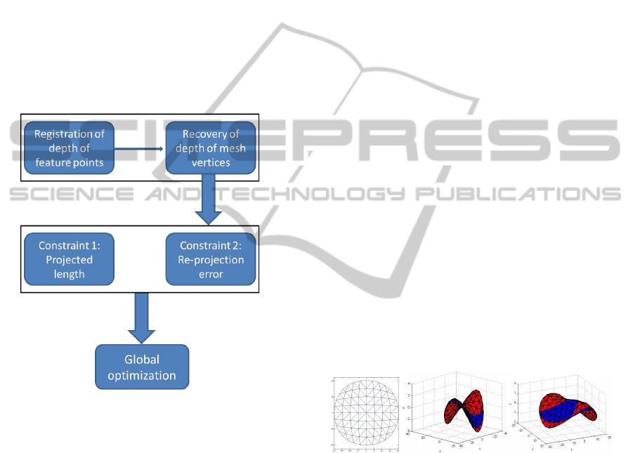
the combined objective function. A block diagram of

the overall structure of the approach is demonstrated

in Figure 2. In our global optimization, we ﬁrst con-

sider a simpliﬁed formulation of the objective func-

tion by excluding the camera motion [R|t]. We in-

clude it back in the second case.

Figure 2: Representation of the approach via block diagram.

4.3.1 Estimation of Structure Only

The constraints are simpliﬁed so that the only un-

known parameter is the structure (we assume that the

camera motion is set to [I|0]).

Orthographic Camera: min

tot



+ m.e



Perspective Camera: min

tot



mpl

+ m.e

mre



4.3.2 Estimation of Both Structure and Camera

Motion

We consider now the full optimization by including

the camera motion.

Orthographic Camera: min

(1:2)

tot



+ m.e



Perspective Camera: min

R,w

tot



mpl

+ m.e

mre



The above optimization problems can be solved us-

ing a non-linear minimization algorithm such as

Levenberg-Marquardt (LMA). The rotation estimates

obtained from this optimization may not satisfy the

orthormality constraints. So, the optimization algo-

rithm must be fed with a good initialization. To pro-

vide initial estimates relatively close to the true ones,

we do the following: if initial guesses for R

(1:2)

and

R are not given, they can be initialized using well-

known methods that attempt to solve for SfM through

non-rigid factorization of



i j



and



i j



from all

frames, for instance, as in (Llado et al., 2005). In

these methods, the factorization is followed by a re-

ﬁnement step to upgrade the reconstruction to metric.

The deformation coefﬁcients w

are initialised to ran-

dom small values. One possible solution to further

meet the rotation constraints is to subsequently apply

Procrustes (Akhter et al., 2009; Xiao et al., 2004).

4.4 Additional Constraint

Non-linear optimization may converge to local min-

ima. The probability of such occurrence can be re-

duced by adding a new regularization term that re-

quires the estimated depth data to be as close to the

measured one as possible. So, we would have:

∑

i=1



[i]

−



(3)

[i]

+ t

(3)



(14)

where v

[i]

is the depth of the vertex i, already recov-

ered and s

[i]

is the 3D position corresponding to the

vertex i. Notice that this regularization is very depen-

dent on the accuracy of v

[i]

Figure 3: Left: A 9 × 9 template mesh with sparse feature

points - Radius = 20 cm. Right: Metric coordinates in cm

- Overlap between the ground-truth shapes (blue) and the

recovered ones (red).

5 EXPERIMENTS

5.1 Synthetic Data

Next, we evaluate the methods described above using

synthetic data. We synthetized a number of frames

of a deforming circle-like paper (radius = 20 cm) ap-

proximated by a 9 × 9 mesh such as the one shown

in Figure 2. The reason to use a circular mesh is that

it is uniform and has a symmetric shape. Therefore,

StructurefromMotion-ToF-aided3DReconstructionofIsometricSurfaces

549

it has similar shapes (up to a rotation) for a number

of different deformations, which, in fact, brings more

complexity to the reconstruction of the right deforma-

tion. The inextensible meshes used for training have

been built using Blender and PCA was then applied

to estimate the deformation model. In order to gen-

erate the input data, we get a sparse set of 3D feature

points (N = 32) well-distributed on the surface of a

reference planar mesh. The camera conﬁguration is

set up in a way that makes the FOV of the ToF cam-

era be part of the FOV of the 2D camera. The exper-

iments are repeated equally for both the orthographic

and perspective cameras. For the perspective case, the

camera model is deﬁned such that the focal length is

f = 500 pixels. The model assumes that the surface is

located 50 cm in front of the cameras (along the opti-

cal axis). The 3D feature points across the surface are

then projected onto the 2D camera and a zero-mean

Gaussian noise with 1-pixel standard deviation (Std)

was then added to these projections. The depth data of

feature points is also generated by adding a zero-mean

Gaussian noise with 0.1 − cm Std. The results of the

quantitative assessment represent an average obtained

from ﬁve deformations randomly selected. By per-

forming 50 trials for each deformation, each average

value was acquired from 250 trials. Two of the esti-

mated deformations and their equivalent ground-truth

are qualitatively illustrated in Figure 3.

Table 1: Preliminary results.

Reconstruction error PRE MRE RotationAccuracy

Our approach - Orthographic 0.0608 0.0755 0.002

Our approach - Perspective 0.0603 0.0751 < 1

◦

5.1.1 Reconstruction Error

The accuracy of the method is reported in terms of

reconstruction errors. The reconstruction errors are

computed with respect to two measures as:

1- Point reconstruction error (PRE): The normal-

ized Euclidean distance between the observed (

)

and estimated (p

) world points according to PRE =

∑

i=1

−

2- Mesh reconstruction error (MRE): The normal-

ized Euclidean distance between the observed (

) and

estimated (v

) mesh vertices, which is computed as

MRE =

∑

i=1

−

The reprojection error of the feature points can be also

regarded as another measure of precision. The accu-

racy of the Stiefel rotation matrix is evaluated based

on the orthonormality constraint as RotationAccuracy =



(2×3)

(2×3)T

− I

(2×2)



. In case of the perspective cam-

era, we compare the axis-angle of the recovered and

ground-truth rotations as RotationAccuracy =



angle −

angle



The quantitative output can be seen in Table 1. Our

approach takes into consideration just few feature

points, though we take advantage of the ToF sensor

to get the depth of them. We have to notice that the

pattern of placement of these points on the surface is

of high importance and we need to examine which

patterns would yield the best results.

Figure 4: Orthographic camera - Left: Average PRE and

average MRE with respect to the increasing noise in image

points. Right: Average PRE and average MRE with respect

to the increasing noise in depth data.

Figure 5: Perspective camera - Left: Average PRE and av-

erage MRE with respect to the increasing noise in image

points. Right: Average PRE and average MRE with respect

to the increasing noise in depth data.

5.1.2 Length of the Edges

When a 3D surface is reconstructed in a truly inexten-

sible way, the length of the recovered edges must be

the same as that of the template edges. So, in order to

see to what extent the lengths remain the same along

the deformation path, we specify a metric to ﬁgure

out the discrepancy between the initial and recovered

lengths as: IsometryExtent =



1 −



∑

i=1





−







× 100%

which has been found to be 95.77% for the proposed

method, which indicates that it preserves the length of

the edges greatly, conﬁrming that isometry constraint

is satisﬁed to a large degree.

5.1.3 The Impact of Noise

Different levels of noise (whether in image points or

in depth data) have been simulated to demonstrate

how robustly the approach reacts to the noise. Each

of these 2 types of noise has been investigated sepa-

rately. Figures 4 and 5 illustrate results for increas-

ing levels of Gaussian noise in feature’s image points,

where the Std varied from 0 to 4 pixels with 1-pixel

increments, together with the reconstruction error for

ICPRAM2014-InternationalConferenceonPatternRecognitionApplicationsandMethods

550

various levels of Gaussian noise in depth of feature

points, with 0.1 − cm increments of Std, which was

computed following the remark that, since the depth

variation of the surface itself is small, the deviations

from the true depth of every 3D point may be very

close together, varying at each trial according to a

Gaussian distribution. From the Figures 4 and 5, we

may draw the conclusion that the white noise does not

make a dramatic impact on the output, ensuring that

the performance remains pretty stable and the algo-

rithm carries on efﬁciently in the face of noise.

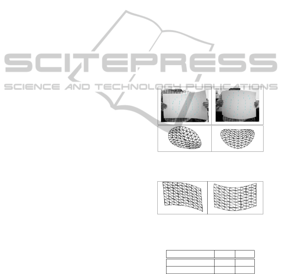
5.2 Real Data

We performed also experiments with real data

recorded using a camera setup comprising a ToF cam-

era and a RGB camera. The camera setup was cali-

brated both internally and externally. Bilinear inter-

polation was applied to estimate the depth of each 2D

point track. We used a piece of cardboard to make

real inextensible deformations and proceeded with the

tracking and matching of few feature points with re-

spect to the reference template using SIFT local fea-

ture descriptor. The same deformation model as the

one acquired in synthetic experiments was employed.

Some deformations and their recovered shapes are

shown in Figure 7. Although it was not possible to

quantitatively assess the results and do benchmark-

ing, the efﬁciency of the approach was visible from

the 3D reconstruction output.

5.2.1 Comparative Evaluations using Motion

Capture Data

Rather than generate the training data synthetically

using Blender, we take advantage of datasets recorded

using Vicon which is able to capture real deforma-

tions accurately. Since the synthetically deformed

meshes might not exactly overlap the real deforma-

tions, we rebuilt the deformation model based on this

real data and redid the experiments. The template

conﬁguration is now composed of equal triangles and

covers a 20 × 20-cm square-like area. As an exam-

ple, the reconstructed surfaces in Figure 7 look bet-

ter than the ones in Figure 6. Consequently, when

learned with real data, the deformation model would

be more robust to the deformations.

As a general rule, two different entities can be com-

pared only when they meet identical conditions which

characterize them. To this end we analyzed the state-

of-art literature and selected the approach described

in (Salzmann et al., 2007). In particular this approach

also uses a triangular mesh and can use the same types

of data sets required by our approach. As a result, to

show how the real training data will inﬂuence the 3D

reconstruction, we performed a set of simulations as

we already did with Blender data and we compare the

performance of our SfM framework to this approach

(where the authors use a second-order cone program

(SOCP) to accomplish the 3D reconstruction of inex-

tensible surfaces). Their approach is known to be very

robust and efﬁcient, where a linear local deformation

model integrates local patches into a global surface

and requires many feature points distributed through-

out the surface. To account for noise in our approach,

like before, a Gaussian noise with 1-pixel Std was

added to the image points and a Gaussian noise with

0.1 − cm Std to the depth data. The SOCP-based ap-

proach was evaluated without noise. We obtained the

results for 5 deformations after having done 50 trials

for each one. From the Table 2, it can be seen that

the result of our approach is comparable to that of the

SOCP-based method. The reconstruction errors are

considerably lower than those in table 1, which may

imply that the use of good-quality real data for train-

ing might improve signiﬁcantly the results.

Figure 6: Real deformations; A 20 × 20-cm square was se-

lected from the intermediate part of the cardboard and the

corresponding circle was reconstructed.

Figure 7: The reconstructed shape of the corresponding

squares in Figure 6.

Table 2: Comparison between the proposed approach and

the SOCP-based one.

Reconstruction error PRE MRE

Our approach 0.0120 0.0185

SOCP-based approach 0.0162 0.0217

6 CONCLUSIONS

In this paper, we have proposed a SfM framework

combining a monocular camera and a ToF sensor to

StructurefromMotion-ToF-aided3DReconstructionofIsometricSurfaces

551

reconstruct surfaces which deform isometrically. The

ToF camera was used to provide us with the depth of

a sparse set of feature points, from which we can re-

cover the depth of the mesh using a multivariate linear

system. The key advantage of the RGB/ToF system is

to beneﬁt from the high-resolution RGB data in com-

bination with the low-resolution depth information.

We proposed an approach to inextensible surface re-

construction, which is formulated as an optimization

problem. Finally, we carried out a set of experiments

showing that the approach generates good results in

cases where 3D points are well-distributed. As next

objective, we will extend the approach to deal with

non-rigid surfaces which are not isometric e.g. con-

formal surfaces and etc.

REFERENCES

Aans, H. and Kahl, F. (2002). Estimation of deformable

structure and motion. Workshop on Vision and Mod-

elling of Dynamic Scenes, ECCV, Denmark.

Akhter, I., Sheikh, Y., and Khan, S. (2009). In defense of

orthonormality constraints for nonrigid structure from

motion. pages 1534–1541. CVPR.

Dai, Y., Li, H., and He, M. (2012). A simple prior-free

method for non-rigid structure-from-motion factoriza-

tion. pages 2018–2025. CVPR.

Del-Bue, A., Llad, X., and Agapito, L. (2006). Non-rigid

metric shape and motion recovery from uncalibrated

images using priors. IEEE Conference on Computer

Vision and Pattern Recognition, New York.

Diebel, J. and Thrun, S. (2005). An application of markov

random ﬁelds to range sensing. Proc. NIPS.

Gay-Bellile, V., Perriollat, M., Bartoli, A., and Sayd, P.

(2006). Image registration by combining thin-plate

splines with a 3d morphable model. International

Conference on Image Processing.

Gumerov, N., Zandifar, A., Duraiswami, R., and Davis, L.

(2004). Structure of applicable surfaces from single

views. European Conference on Computer Vision.

Kim, H., Tai, Y.-W., and Brown, M. (2011). High quality

depth map upsampling for 3d-tof cameras. pages 1623

– 1630. Inso Kweon Computer Vision (ICCV), IEEE

International Conference, Barcelona.

Kim, Y., Theobalt, C., Diebel, J., Kosecka, J., Miscusik, B.,

and Thrun, S. (2009). Multi-view image and tof sensor

fusion for dense 3d reconstruction. pages 1542–1549.

Computer Vision Workshops (ICCV Workshops).

Llado, X., Bue, A., and Agapito, L. (2005). Non-rigid 3d

factorization for projective reconstruction. BMVC.

Metaxas, D. and Terzopoulos, D. (1993). Constrained de-

formable superquadrics and nonrigid motion tracking.

PAMI 15, pages 580–591.

Paladini, M., Bue, A., Stosic, M., Dodig, M., Xavier, J., and

Agapito, L. (2009). Factorization for non-rigid and

articulated structure using metric projections. page

28982905. Proc. IEEE Conf. on Computer Vision and

Pattern Recognition.

Perriollat, M., Hartley, R., and Bartoli (2010). Monocu-

lar template-based reconstruction of inextensible sur-

faces. International Journal of Computer Vision.

Prasad, M., Zisserman, A., and Fitzgibbon, A. (2006). Sin-

gle view reconstruction of curved surfaces. pages

1345–1354. IEEE Conference on Computer Vision

and Pattern Recognition.

Salzmann, M. and Fua, P. (2007). Reconstructing sharply

folding surfaces: A convex formulation. IEEE Con-

ference on Computer Vision and Pattern Recognition.

Salzmann, M., Hartley, R., and Fua, P. (2007). Convex op-

timization for deformable surface 3-d tracking. IEEE

International Conference on Computer Vision.

Salzmann, M., Moreno-Noguer, F., Lepetit, V., and Fua, P.

(2008). Closed-form solution to non-rigid 3d surface

registration. pages 581–594. European Conference on

Computer Vision.

Shen, S., Shi, W., and Liu, Y. (2010). Monocular 3-d

tracking of inextensible deformable surfaces under l2-

norm. IEEE Transactions on Image Processing 19,

pages 512–521.

Srivastava, S., Saxena, A., Theobalt, C., and Thrun, S.

(2009). Rapid interactive 3d reconstruction from a

single image. In VMV, pages 19–28.

Torresani, L., Hertzmann, A., and Bregler, C. (2003).

Learning non-rigid 3d shape from 2d motion. NIPS,

pages 580–591.

White, R. and Forsyth, D. (2006). Combining cues: Shape

from shading and texture. CVPR.

Xiao, J., x. Chai, J., and Kanade, T. (2004). A closed-

form solution to non-rigid shape and motion recovery.

pages 573–587. ECCV.

Yang, R., Davis, J., and Nister, D. (2007). Spatial-depth su-

per resolution for range images. pages 1–8. Computer

Vision and Pattern Recognition, CVPR ’07. IEEE

Conference, Minneapolis, MN.

Zhou, H., Li, X., and Sadka, A. (2012). Nonrigid structure-

from-motion from 2-d images using markov chain

monte carlo. 14(1):168–177.

ICPRAM2014-InternationalConferenceonPatternRecognitionApplicationsandMethods

552