
Modified Fuzzy C-Means as a Stereo Segmentation Method
Michal Krumnikl, Eduard Sojka and Jan Gaura
V
ˇ
SB - Technical University of Ostrava, Faculty of Electrical Engineering and Computer Science,
17. listopadu 15, 708 33 Ostrava-Poruba, Czech Republic
Keywords:
Fuzzy C-Means, Segmentation, Stereo Matching, Disparity.
Abstract:
This paper presents an extension to the popular fuzzy c-means clustering method by introducing an additional
disparity cue. The creation of the clusters is driven by a degree of the stereo match and thus is able to separate
the objects based on their different colour and spatial depth. In contrast to the other popular approaches,
the clustering is not performed on the individual input images, but on the stereo pair, and takes into account
the matching properties. The algorithm is capable of producing the segmentations, as well as the disparity
maps. The results of this algorithm show that the proposed method can improve the segmentation, under the
condition of having the stereo image pair of the segmented scene.
1 INTRODUCTION
This paper presents an extension to the popular fuzzy
c-means clustering method by introducing an addi-
tional disparity cue. The proposed approach is in-
tended to improve the segmentation, under the condi-
tion of having the stereo image pair of the segmented
scene. Beside the segmentation with additional depth
constraint, this method is also capable of producing
the disparity map of the input image pair and hence
can be considered as a form of the stereo matching
algorithm.
In the following text, we will describe the adap-
tation of the fuzzy c-means algorithm to perform the
clustering in space extended by the dimension of the
disparity. The creation of the clusters will be driven
by a degree of the stereo match (this measure will be
described later on). An attractive aspect of this strat-
egy is that we are able to take advantage of known
number of depth levels or objects (if this information
is available).
The motivation for our work was to provide an al-
gorithm that can separate objects based on their differ-
ent colour and spatial depth. We regard this method
as more suitable in specific cases (will be described
later on) than the segmentation with the final disparity
maps of the stereo matching algorithms. The distance,
based on both dissimilarities (spatial and colour), pro-
vide more sensitive segmentation (especially on seg-
ment borders) than the segmentation performed on the
filtered disparity maps which contain only the best
matches, and do not take into account segment prop-
erties. The algorithm was originally developed for a
very specific purpose – the segmentation of the moss
clusters (as a part of a biological research involving
these species). Therefore, we have tested and evalu-
ated the algorithm mainly on the ”Map” dataset, in-
troduced in (Szeliski and Zabih, 2000), as it strongly
resembles the stone structures which are frequently
covered by the moss layers. However, as we will show
in the next paragraphs, the algorithm can be used in
more general cases.
The clustering technique is usually described as a
process of forming partitions from a data set on the
basis of a performance function, also known as an
objective function. The underlying idea of our algo-
rithm is to consider the disparity space (e.g., in dispar-
ity maps) as a specific type of the data set, consisting
of clusters representing the three dimensional objects
of the scene. The fuzzy c-means algorithm has al-
ready been used to create the segmentations based on
the depth information or disparity maps, e.g., (Ntal-
ianis et al., 2002; Aik and Choon, 2011), and was
also adapted to incorporated the spatial neighbour-
hood information, e.g., (Liew et al., 2000; Chuang
et al., 2006; Meena and Raja, 2013), but in all these
approaches, the algorithms were run on the input data
already containing the depth information for each pro-
cessed point. Our algorithm does not need the depth
information in advance, since it calculates it itself by
means of the stereo matching.
The basic idea of using the clustering technique
together with the stereo matching process was intro-
duced in (Tao et al., 2001; Bleyer and Gelautz, 2004)
40
Krumnikl M., Sojka E. and Gaura J..
Modified Fuzzy C-Means as a Stereo Segmentation Method.
DOI: 10.5220/0004793000400047
In Proceedings of the 3rd International Conference on Pattern Recognition Applications and Methods (ICPRAM-2014), pages 40-47
ISBN: 978-989-758-018-5
Copyright
c
2014 SCITEPRESS (Science and Technology Publications, Lda.)

and further developed in (Zitnick and Kang, 2007;
Tombari et al., 2007; Taguchi et al., 2008; Liu et al.,
2009). Compared to these, our approach differs in
several aspects. The clustering is not performed on
the individual input images, but on both stereo images
simultaneously, and takes into account the matching
properties. In each step, the clusters are adjusted to
minimize the matching cost.
In the following sections, we will introduce and
describe each particular step used in the proposed
modification of the fuzzy c-means algorithm and pro-
vide the results obtained using this approach.
2 FUZZY C-MEANS
Let us briefly introduce the original method. Fuzzy
c-means is a widely used clustering technique, de-
veloped by (Dunn, 1973) and improved by (Bezdek,
1981). It is based on a standard least squared error
model that generalizes an earlier and popular non-
fuzzy c-means mode (Miyamoto et al., 2008). Fuzzy
c-means can be generalized in many ways to include,
e.g., Minkowski, Hamming, Canberrar or hybrid dis-
tances.
The fuzzy c-means algorithm attempts to partition
a collection of n data points {x
k
}
n
k=1
into a collection
of c fuzzy clusters (represented by the cluster centres)
on the basis of a distance d between the cluster cen-
tre and the data point. The algorithm is minimizing
the objective function J(U,V ), where V = (v
1
, . . . , v
c
)
is the set of cluster centres and U = [u
ki
] is the n × c
membership matrix. The space of all possible values
of U is denoted as U
f
. The elements of the matrix
U are organized as follows. The column i gives the
membership of all n input data points (rows) in the
cluster i for i = 1. . . c. The u
ki
stands for the mem-
bership of the k-th point of the i-th cluster. The idea
is that the closer the data point is to the cluster cen-
tre, the larger is its membership value towards that
specific cluster. Consequently, the sum of all mem-
berships of the data point across all clusters is equal
to one. The fuzzy membership is formally given by
the following constraint
U
f
= {U = (u
ki
) :
c
∑
j=1
u
k j
= 1, 1 ≤ k ≤ n;
u
ki
∈ [0, 1], 1 ≤ k ≤ n, 1 ≤ i ≤ c}. (1)
The minimized objective function J(U,V ) is defined
as (Bezdek, 1981)
J(U,V ) =
c
∑
i=1
n
∑
k=1
(u
ki
)
m
d(x
k
, v
i
), (1 ≤ m ≤ ∞), (2)
where u
ki
is a degree of membership of x
k
in the clus-
ter i, and v
i
represents the centre of the cluster. The
parameter m is called the weighting exponent of the
model. For m = 1, the memberships converge to 0 or
1, producing a crisp partitioning. The best choice for
m is probably in the interval [1.5, 2.5], where m = 2
is the most common choice (Pal and Bezdek, 1995).
The distance d(x
k
, v
i
) represents (usually) Euclidean
distance between the k-th data point and the i-th clus-
ter centre.
We should notice that the minimization of the ob-
jective function J(U,V ) is not an exact minimization
but an iteration procedure of so called ”alternate min-
imization”. In essence, the algorithm is searching for
a local optimal solution, which we will denote with
stripe (e.g.,
¯
U). The overall iterative process may be
summarised as follows.
Algorithm Steps
1. Initialize the matrix U by randomly generated
u
ki
membership coefficients for all cluster centres
¯
V = ( ¯v
1
, . . . , ¯v
c
).
2. Find the optimal U by iteratively calculating
¯
U =
arg min
U∈U
f
J(U,
¯
V ). The following solution can be
derived using the Lagrange multiplier method
(Miyamoto et al., 2008)
¯u
ki
=
"
c
∑
j=1
d(x
k
, ¯v
i
)
d(x
k
, ¯v
j
)
2
m−1
#
−1
, (x
k
6= v
i
). (3)
The solution for (x
k
= v
i
) is obviously ¯u
ki
= 1.
3. Find the optimal V by calculating
¯
V = argmin
V
J(
¯
U,V ). The solution is com-
puted by differentiating J with respect to V
(Miyamoto et al., 2008):
¯v
i
=
n
∑
k=1
( ¯u
ki
)
m
x
k
n
∑
k=1
( ¯u
ki
)
m
. (4)
4. Repeat from step 2 until
¯
U and
¯
V is convergent.
The convergence is achieved when max
k,i
| ¯u
ki
−u
ki
| < ε,
where ¯u is the new solution, u is the value from the
previous iteration and ε is a small positive number, the
threshold. Alternatively, we can use max
1≤i≤c
k ¯v
i
− v
i
k <
ε as a convergence condition.
ModifiedFuzzyC-MeansasaStereoSegmentationMethod
41

Figure 1: Illustration of the rationale behind the algorithm.
The left figure shows the coloured disparity levels of the
dataset (Scharstein and Szeliski, 2002), while the right one
depicts the original pixel colours. The algorithm is based on
the observation that the objects share the similar disparity,
as well as similar colour. This can be clearly seen on the red
lamp in the foreground or the white statue on the left.
3 INTRODUCING THE
MATCHING CONSTRAINT TO
FUZZY C-MEANS
In a simplified way, we can say that the original fuzzy
c-means algorithm (when used in image processing)
is usually based only on the pixel positions and their
intensities (colours). In our approach, we have ex-
tended this algorithm to include the matching con-
straints. First, by expanding the dimension of the data
vector to include the disparity (depth), and then, by
evaluating the dissimilarity of the stereo pair (which
will be explained later).
As stated in Section 2, the algorithm attempts to
partition the elements with respect to a given crite-
rion, defined as a degree of belonging that is related
inversely to the distance. However, for the depth
segmentation, we need to add additional components
measuring the intensity (colour) difference between
the point and its supposed projection and the distance
between the point disparity and the disparity of its
supposed cluster. In that way, we associate the clus-
ters with the disparity space. Therefore, we have to
define the vector of the cluster centre as
v = (v
X
, v
Y
, v
I
, v
D
), (5)
where v
X
,v
Y
stand for the spatial position, v
I
for the
brightness and v
D
for the disparity value. For the clar-
ity, the capitalized subscripts, X, Y, I and D, are used
to indicate the vector elements. The small subscripts
will later be used to specify a particular vector from
the set.
Our new membership function takes into account
the dissimilarity of the left image pixel and the right
image pixel shifted by the average cluster disparity.
We use the disparity in the similar fashion as the in-
tensity, grouping the pixels sharing the same, or al-
most the same disparity value (see Figure 1). For this,
Figure 2: Visualisation of the data points and their clusters
taken from our experiments. The points on the left figure are
coloured according to the disparity levels associated with
them. The right figure shows their real colour. The both
figures shows the depth levels as obtained from the calcu-
lations of the proposed modification of the fuzzy c-means
algorithm.
we need to adapt the membership function to penal-
ize the pixels having the incorrect match (not similar
to their projections on the other image) and provide
the way of measuring the distance between the clus-
ter centres and pixels with associated disparity value.
We propose the use of the extended vector space
model with the additional dimensions reflecting the
disparity and pixel dissimilarity in the stereo image
pair. The distance in the proposed vector space is, for
clarity, separated into the two components (d and d
s
),
described later on. The proposed fuzzy stereo parti-
tioning is carried out using the following membership
function (the subscripts k, i, j are the indexes)
¯u
ki
=
c
∑
j=1
d
2
(x
k
, ¯v
i
) + d
2
s
(x
k
, ¯v
i
)
d
2
(x
k
, ¯v
j
) + d
2
s
(x
k
, ¯v
j
)
1
m−1
−1
, (x
k
6= v
i
).
(6)
The membership ¯u
ki
is related inversely to the dis-
tance between the processed point and the cluster cen-
tre (as calculated in the previous iteration). The new
term d
s
reflects the correctness of the stereo match
between the pixel of the left (φ
L
) and its projection on
the right (φ
R
) image (the subscripts X,Y, D denotes
the vector elements):
d
2
s
(x, v) = λ
m
(φ
L
(x
X
, x
Y
) − φ
R
(x
X
+ v
D
, x
Y
))
2
, (7)
where x is the data point (vector) and v is the cluster
centroid. The uppercase subscript of the vector de-
notes its component. The constant λ
m
stands for the
weight of the matching term. For φ
L
and φ
R
we as-
sume the rectified images. It is possible to replace the
difference φ
L
(x
X
, x
Y
) − φ
R
(x
X
+ v
D
, x
Y
) by the differ-
ence of the aggregating windows (SAD, SSD, etc.),
but as the aggregation of the pixels is inherently given
by the fuzzy c-means, it does not provide any further
advantage and even worsens the results by blurring
ICPRAM2014-InternationalConferenceonPatternRecognitionApplicationsandMethods
42
the edges. The distance d(x, v) is calculated (as in
original method) using the Euclidean distance:
d
2
(x, v) = λ
i
(x
I
− v
I
)
2
+ λ
d
(x
D
− v
D
)
2
+
λ
s
(x
X
− v
X
)
2
+ λ
s
(x
Y
− v
Y
)
2
, (8)
where x
X
, x
Y
are the pixel coordinates, x
I
colour in-
tensity and x
D
is the disparity value. When compared
to the original method, we have added the term mea-
suring the disparity distance of the processed point
and the cluster (see Figure 2). For the pixel disparity
x
D
we can take an initial guess since, as we will show
later, the algorithm is quite insensitive to this value.
Basically, it only helps in the beginning to form the
initial clusters. The values λ
i
, λ
d
and λ
s
denote the
intensity, disparity and spatial weights. The effects of
these weights are discussed with results (Section 4).
The iteration steps remain the same as in Section
2. The outline of the algorithm can be summarized as
follows: (i) choose the proper parameters, especially
the number of clusters (discussed in Section 3.1), (ii)
to each point assign random cluster membership co-
efficients, (iii) in each iteration compute the centroid
for each cluster (Eq. 4), followed by the computa-
tion of the membership coefficients for all points (Eq.
6). Repeat this step until the algorithm has converged.
Finally, create the output disparity map based on the
cluster disparities (iv).
The algorithm was tested on several types of real
images (depicting the processed botanical samples)
and also on the standard dataset used for the evalua-
tion of the stereo matching algorithms (Scharstein and
Szeliski, 2002). While our approach is not intended to
be used as the general purpose stereo matching algo-
rithm, we would like to give the reader an opportunity
to examine the results in the standard stereo matching
benchmark tests (see Section 4).
3.1 Cluster Count Problem
The disadvantage of the fuzzy c-means (as well as k-
means) is the result dependency on the initial choice
of weights. This is also true for our method. De-
spite the algorithm minimizes the intra-cluster vari-
ance, calculated minimum is still only a local mini-
mum. But more serious problem of the fuzzy c-means
algorithm is that it requires the number of clusters to
be known in advance.
The correct choice of the cluster count is ambigu-
ous, with interpretations depending on the shape and
scale of the data point distribution in the input data set
and the desired resolution. This may seem as a disad-
vantage for general settings, but may be an advantage
for special cases, where the number of segments or
number of disparity planes is already known. For ex-
ample, in Figure 3 the box is the only object in the
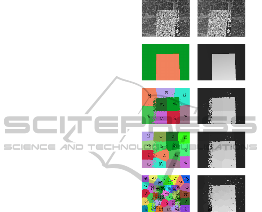
(a) Left Image (b) Right Image
(c) Segments (d) Truth Disparity
(e) Segm. Results (9 s.) (f) Segm. Disparity (9 s.)
(g) Segm. Results (15 s.) (h) Segm. Disparity (15 s.)
(i) Segm. Results (40 s.) (j) Segm. Disparity (40 s.)
Figure 3: The influence of the cluster count on the out-
put disparity map. For better reading, the segments are
coloured, numbered (number in brackets) and marked with
their disparity values (the value below the number in brack-
ets). The input (reference) images (a, b) and the ground
truth disparity map (d) and its segments (c) are provided in
the first row. The subfigures (e, g, i) show the results of
the modified fuzzy c-means algorithm set to 9, 15 and 40
segments. The left subfigures show the segments, while the
right ones (f, h, j) show the disparity maps obtained from
the segments disparity values.
foreground, and can be easily represented by only a
small number of segments. As you can see, with only
a few clusters, we are able to acquire very precise dis-
parity map and by increasing the number of the seg-
ments, we are able to capture even smaller changes
in the disparity gradient (the box in the example is
slightly tilted). We can say that by choosing the num-
ber of clusters, we can set, whether we are more in-
terested in large segments covering the whole objects,
or small fine-grained parts.
ModifiedFuzzyC-MeansasaStereoSegmentationMethod
43
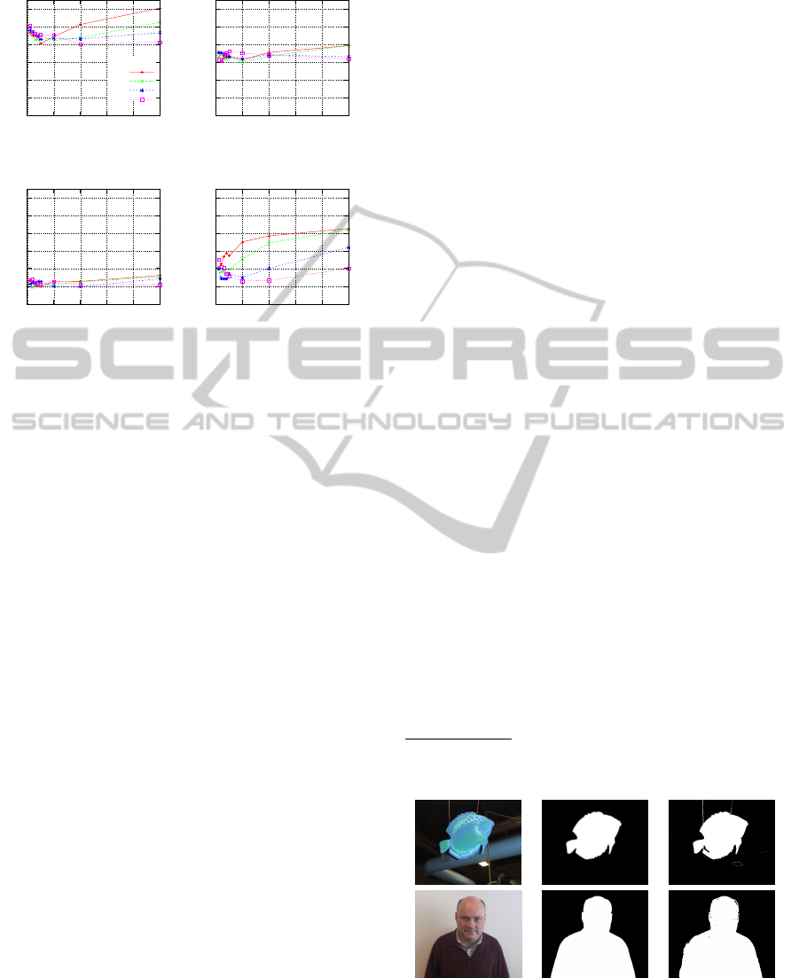
0
10
20
30
40
50
60
0 0.1 0.2 0.3 0.4 0.5
PER [%]
λ
s
Cones
λ
d
0.5
1.0
2.0
5.0
0
10
20
30
40
50
60
0 0.1 0.2 0.3 0.4 0.5
PER [%]
λ
s
Teddy
0
10
20
30
40
50
60
0 0.1 0.2 0.3 0.4 0.5
PER [%]
λ
s
Tsukuba
0
10
20
30
40
50
60
0 0.1 0.2 0.3 0.4 0.5
PER [%]
λ
s
Venus
Figure 4: The algorithm results achieved with different
disparity and spatial weights (λ
d
and λ
s
). The algorithm
was set to generate 100 segments. The different disparity
weights (λ
d
) are represented by the different line colours.
The significant effects of the disparity weight (λ
d
) can be
seen only on the images containing the planar objects (e.g.,
the ”Venus” pair).
The results of our approach surpass (but only for
the specific types of scenes, similar to the sample im-
ages) the performance of the majority of the standard
state-of-the-art algorithms (see Table 1, ”Map” col-
umn). However, due to the algorithm specialization,
it is less suitable for the other types of scenes. But
still, the additional cue improves the segmentation re-
sults.
4 TESTS AND RESULTS
This section describes the experiments and shows the
results confirming the anticipated segmentation fea-
tures and proper depth discrimination.
First, we have performed the tests on the images
fulfilling the assumptions, we made in the beginning
– the scenes with only a few objects, each having al-
most the flat depth. The ”Map” dataset (Figure 3)
complies with these requirements. The results for this
specific dataset are very satisfactory (Table 1, column
”Map”); however, the results for the other types of
image pairs (from the dataset) are not very encourag-
ing. We do not consider this as a disadvantage, since
the intentions of this algorithm are different than the
general purpose stereo matching algorithms. The ex-
planation for the results on the other samples is that
these pairs violate the initial presumptions of our al-
gorithm; the scenes contain a lot of objects with fine-
grained disparity. The limits of our algorithm – the
number of clusters and plane disparities – do not offer
many opportunities for improvements in such general
cases.
To illustrate the algorithm performance on the im-
ages with optimal object configurations, we have cho-
sen several samples from the Adobe Open Source
Data Sets
1
. The data set contains stereo images and
ground truth segmentation of the foreground object.
The results of the selected images are visible on Fig-
ure 5. We have to point out that these images illustrate
the optimal cases.
Nevertheless, we have also performed the tests
on the images that are not very suitable for our ap-
proach. The absolute results with the comparison of
the other algorithms are shown in Table 1. The eval-
uation has been performed on the Middlebury dataset
(Scharstein and Szeliski, 2002). The full list of al-
gorithms is available on the Middlebury stereo vision
website. While our algorithm is not the typical stereo
matching algorithm, due to the lack of more suitable,
generally accepted dataset for segmenting the stereo
images, we decided to perform the tests on these im-
ages. The parameters were maintained the same for
all images – cluster count n = 200, λ
d
= 1.0, λ
s
= 0.1,
λ
i
= 0.05, and λ
m
= 0.1.
The proposed algorithm converges approximately
after 15 iterations on all images of the given set. The
outputs with 100 segments are displayed in Figure 6
(evaluated outputs with 200 segments were not used
for the illustration purposes, due to the hard distin-
guishability of the small clusters). The images in the
upper row show the segments. The disparity maps
obtained from the segment properties are displayed
below. As you can see, the proposed algorithm is
capable of obtaining the disparity maps of more so-
1
http://sourceforge.net/adobe/adobedatasets/
Left Ground Truth Results
Figure 5: Segmentation results of two samples from the
Adobe Open Source Data Sets. These samples illustrate the
ideal configurations for the proposed algorithm – raised flat
foreground objects.
ICPRAM2014-InternationalConferenceonPatternRecognitionApplicationsandMethods
44
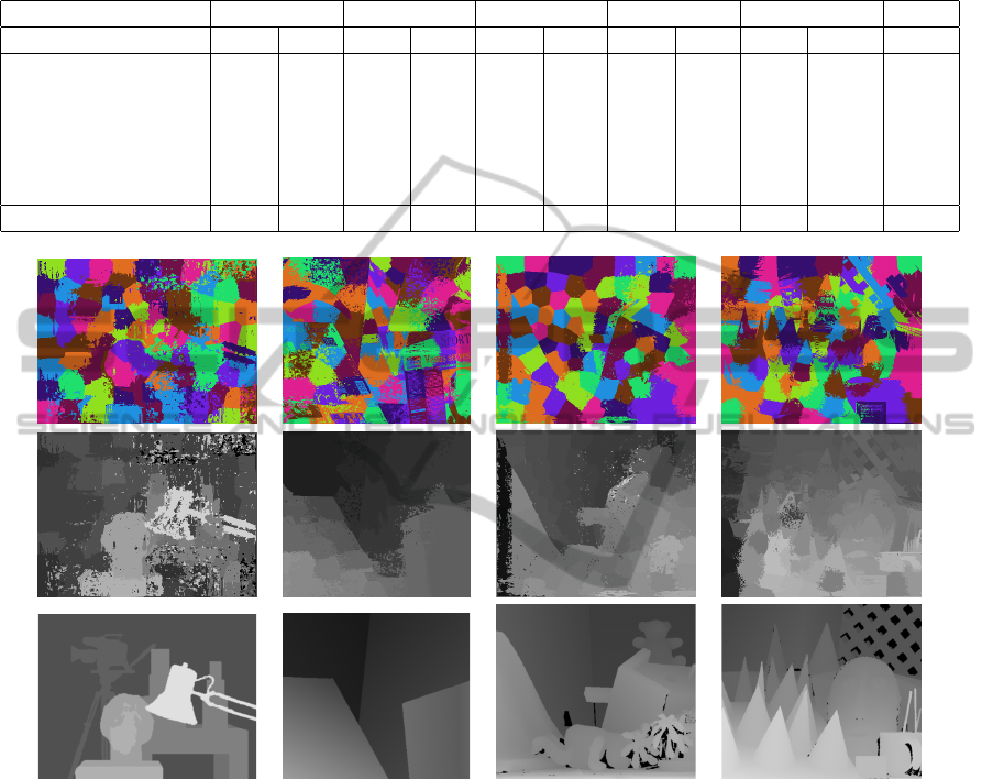
Table 1: The performance of the modified fuzzy c-means algorithms according the Middlebury stereo test bed (Scharstein and
Szeliski, 2002). The overall performance is measured by the percentage of bad pixels in the non-occluded areas (nocc). The
performance measured on the whole image (all) is provided as well. Our algorithm is denoted as FZ. The total cluster count
was set to 200. In order to give a better idea of the performance of our methods compared to the state-of-the-art algorithms,
we have included the results of the selected algorithms from the Middlebury evaluation.
Tsukuba Venus Teddy Cones Map
Algorithm nocc all nocc all nocc all nocc all nocc all avg
(Hirschm
¨
uller, 2006) 2.61 3.29 0.25 0.57 5.14 11.8 2.77 8.35 1.09 2.82 5.33
(Klaus et al., 2006) 0.97 1.75 0.16 0.33 6.47 10.7 4.79 10.7 3.39 5.79 5.85
(Hirschm
¨
uller, 2005) 3.26 3.96 1.00 1.57 6.02 12.2 3.06 9.75 1.12 2.97 6.09
(Kim et al., 2003) 1.94 4.12 1.79 3.44 16.5 25.0 7.70 18.2 0.74 6.82 11.51
(Cox et al., 1996) 4.12 5.04 10.1 11.0 14.0 21.6 10.5 19.1 6.04 12.12 13.77
Standard SSD 5.23 7.07 3.74 5.16 16.5 24.8 10.6 19.8 8.49 14.57 14.28
FZ 12.7 14.3 12.5 13.5 32.3 37.8 32.0 36.9 0.72 7.17 21.93
Figure 6: The images show the disparity and cluster maps obtained for the default Middlebury dataset using our expanded
fuzzy c-means algorithm ( f z). The ground truth data are provided in the last row. As you can see, the output disparity maps
are not as good as the results from the ”Map” dataset (Figure 3). The reason for that is the Middlebury dataset contains images
with lot of details and a set of various objects, which contradicts the initial algorithm assumptions. In order to improve the
performance it is necessary to significantly increase the number of the clusters, which consequently leads to a much longer
processing time. Unfortunately, this still does not guarantee for all inputs the results comparable to the best algorithms.
phisticated scenes, but not at the level of detail as the
generally used stereo matching approaches.
To increase the overall performance, it is possi-
ble to increase the number of clusters, which in re-
sult leads to a more grained segmentation, where each
segment can have different disparity. The drawback
of a huge number of clusters is the increasing com-
putational time. At the certain level, the additional
increasing of cluster count starts to be inefficient. We
have used no more than 200 segments.
During the development, we have also performed
several experiments to investigate the effects of the
algorithm parameters on the segmentation perfor-
mance. The parameter settings may vary from sce-
nario to scenario, but generally, only two parameters
appear to be particularly influential - the spatial and
disparity weight (λ
s
and λ
d
). Figure 4 shows the influ-
ence of these weights on the output segmentation con-
sisting of 100 segments. The experiment showed the
significant effect of the disparity weight (λ
d
) mainly
on the images containing the planar objects (e.g., the
”Venus” pair). This is a predicted behaviour as our
ModifiedFuzzyC-MeansasaStereoSegmentationMethod
45

(a) Left Source Image (b) Segments Brightness
(c) Segments Disparity (d) Output Segments
Figure 7: The segmentation results of the moss sample us-
ing the modified fuzzy c-means algorithm (Section 3). The
figure shows (from left to right, up to down): the left im-
age of the input pair depicting the moss layers on the stone
base, the segments coloured according the average colour,
the segments coloured according the disparity and the visu-
alization of the clusters itself. As you can see, our modi-
fication of the fuzzy c-means still retains the properties of
the original algorithm and in addition provides the disparity
values.
algorithm favours planar disparities. On an exam-
ple of ”Venus” pair, you can see that the increasing
disparity weight forces the algorithm to create seg-
ments with less disparity deviations from the cluster
centroid, leading to the better results. However, for
images not containing such objects (e.g., ”Teddy” or
”Tsukuba”) the change in these parameters has only a
small impact on the results. We have not evaluated all
possible parameter configurations for all dataset im-
ages, but empirically, we can say that the best results
were achieved with λ
s
= 0.1. Increasing this value
forced the algorithm to create too compact clusters
and, vice versa, decreasing λ
s
caused merging too dis-
tant pixels into one cluster.
In the application that the algorithm was originally
developed for, it was important to separate the layer
of the base (usually the stone) and the layer above,
formed by the moss structures. An example is illus-
trated in Figure 7. As you can see, the resulting seg-
mentation strongly benefits from the inherit features
of the algorithm. The design of the algorithm was
strongly driven by the expected look of the captured
samples.
5 CONCLUSIONS
In this paper, we have presented a modification of the
fuzzy c-means algorithm. The fuzzy c-means algo-
rithm is one of the most popular clustering techniques
in image processing. In the past, it has been modi-
fied in many ways to take into account different con-
straints. In our case, we have added an additional
disparity constraint and examined its impact on the
segmentation performance and depth discrimination.
In the context of the image segmentation, we see the
advantage of the proposed joint analysis using bright-
ness and depth constraints. We believe, such combi-
nation improves the segmentation by creating edges
not only in places where brightness changes abruptly
but also in places of the depth discontinuities. Ob-
jects of the similar colour in different depths may be
connected by the classical algorithm but with an ad-
ditional depth constraint they are separated correctly.
The motivation was to develop a segmentation
technique that can be used in cases, where we have
the possibility of obtaining the stereo images and, in
such way, improve the segmentation by applying ad-
ditional depth information. In the biological applica-
tion (the segmentation of the moss layers), the method
provided better results than the standard fuzzy c-mean
algorithm. As the algorithm was intended for this
specific application, we have mainly tested and evalu-
ated the algorithm on the datasets that resemble stone
structures (e.g., the standard ”Map” dataset). For such
cases, the algorithm provides very good results.
The paper proposed the method that improves the
segmentation in cases where the pixel intensities are
not sufficient for correct segmentation and the stereo
images are available. This area of research, however,
still offers some space for improvements. Presently,
we will focus on improving the results by tuning the
distance weights. The aim is to create a method that
can automatically adapt the weight variables accord-
ing to the input dataset. Similar approaches were al-
ready published for the closely related k-means clus-
tering, e.g. (Modha and Spangler, 2003; Huang et al.,
2005), and should be applicable (with small modifi-
cations) to the fuzzy c-means.
ACKNOWLEDGEMENTS
This work was partially supported by the SGS grant
No. SP2014/170 of V
ˇ
SB - Technical University of
Ostrava, Faculty of Electrical Engineering and Com-
puter Science.
ICPRAM2014-InternationalConferenceonPatternRecognitionApplicationsandMethods
46

REFERENCES
Aik, L. E. and Choon, T. W. (2011). Enhancing passive
stereo face recognition using pca and fuzzy c-means
clustering. International Journal of Video and Image
Processing and Network Security, 11(4):1–5.
Bezdek, J. C. (1981). Pattern Recognition with Fuzzy Ob-
jective Function Algorithms. Kluwer Academic Pub-
lishers, Norwell, MA, USA.
Bleyer, M. and Gelautz, M. (2004). A layered stereo algo-
rithm using image segmentation and global visibility
constraints. In Proceedings of the IEEE International
Conference on Image Processing, pages 2997–3000.
Chuang, K.-S., Tzeng, H.-L., Chen, S., Wu, J., and Chen,
T.-J. (2006). Fuzzy c-means clustering with spatial
information for image segmentation. Computerized
Medical Imaging and Graphics, 30(1):9 – 15.
Cox, I. J., Hingorani, S. L., Rao, S. B., and Maggs, B. M.
(1996). A maximum likelihood stereo algorithm.
Computer Vision and Image Understanding, 63:542–
567.
Dunn, J. C. (1973). A Fuzzy Relative of the ISODATA Pro-
cess and Its Use in Detecting Compact Well-Separated
Clusters. Journal of Cybernetics, 3(3):32–57.
Hirschm
¨
uller, H. (2005). Accurate and efficient stereo pro-
cessing by semi-global matching and mutual informa-
tion. In Proceedings of the IEEE Conference on Com-
puter Vision and Pattern Recognition, pages 807–814.
Hirschm
¨
uller, H. (2006). Stereo vision in structured envi-
ronments by consistent semi-global matching. In Pro-
ceedings of the IEEE Conference on Computer Vision
and Pattern Recognition, volume 2, pages 2386–2393.
IEEE Computer Society.
Huang, J., Ng, M., Rong, H., and Li, Z. (2005). Automated
variable weighting in k-means type clustering. Pat-
tern Analysis and Machine Intelligence, IEEE Trans-
actions on, 27(5):657–668.
Kim, J., Kolmogorov, V., and Zabih, R. (2003). Visual
Correspondence Using Energy Minimization and Mu-
tual Information. In Proceedings of the IEEE Inter-
national Conference on Computer Vision, volume 2,
pages 1033–1040.
Klaus, A., Sormann, M., and Karner, K. F. (2006).
Segment-based stereo matching using belief propaga-
tion and a self-adapting dissimilarity measure. In Pro-
ceedings of the IEEE Conference on Computer Vision
and Pattern Recognition, volume 3, pages 15–18.
Liew, A. W. C., Leung, S. H., and Lau, W. H. (2000). Fuzzy
image clustering incorporating spatial continuity. In
IEEE Proceedings of the Vision, Image and Signal
Processing, volume 147, pages 185–192.
Liu, T., Zhang, P., and Luo, L. (2009). Dense stereo
correspondence with contrast context histogram,
segmentation-based two-pass aggregation and occlu-
sion handling. In Proceedings of the Pacific-Rim Sym-
posium on Image and Video Technology, pages 449–
461.
Meena, A. and Raja, R. (2013). Spatial fuzzy c means
pet image segmentation of neurodegenerative disor-
der. CoRR, abs/1303.0647.
Miyamoto, S., Ichihashi, H., and Honda, K. (2008). Al-
gorithms for Fuzzy Clustering: Methods in C-Means
Clustering with Applications. Studies in Fuzziness
and Soft Computing. Springer-Verlag.
Modha, D. and Spangler, S. (2003). Feature weighting in
k-means clustering. In Machine Learning, volume 52,
pages 217–237.
Ntalianis, K. S., Doulamis, A., Doulamis, N., and Kollias,
S. (2002). Unsupervised segmentation of stereoscopic
video objects: investigation of two depth-based ap-
proaches. In Proceedings of the 14th International
Conference of Digital Signal Processing, 2002, vol-
ume 2, pages 693–696.
Pal, N. and Bezdek, J. (1995). On cluster validity for the
fuzzy c-means model. IEEE Transactions on Fuzzy
Systems, 3(3):370–379.
Scharstein, D. and Szeliski, R. (2002). A taxonomy and
evaluation of dense two-frame stereo correspondence
algorithms. International Journal of Computer Vision,
47(1-3):7–42.
Szeliski, R. and Zabih, R. (2000). An experimental compar-
ison of stereo algorithms. In Proceedings of the Inter-
national Workshop on Vision Algorithms: Theory and
Practice, pages 1–19.
Taguchi, Y., Wilburn, B., and Zitnick, C. L. (2008). Stereo
reconstruction with mixed pixels using adaptive over-
segmentation. In Proceedings of the IEEE Conference
on Computer Vision and Pattern Recognition, pages
1–8.
Tao, H., Sawhney, H. S., and Kumar, R. (2001). A global
matching framework for stereo computation. In Pro-
ceedings of the IEEE International Conference on
Computer Vision, pages 532–539.
Tombari, F., Mattoccia, S., and di Stefano, L. (2007).
Segmentation-based adaptive support for accurate
stereo correspondence. In Proceedings of the Pacific-
Rim Symposium on Image and Video Technology,
pages 427–438.
Zitnick, C. L. and Kang, S. B. (2007). Stereo for image-
based rendering using image over-segmentation. In-
ternational Journal of Computer Vision, 75(1):49–65.
ModifiedFuzzyC-MeansasaStereoSegmentationMethod
47
