
Evolutionary Fuzzy Rule Construction for Iterative Object Segmentation
Junji Otsuka and Tomoharu Nagao
Department of Information Media and Environment Sciences, Yokohama National University, Yokohama, Japan
Keywords:
Fuzzy Inference, Genetic Algorithm, Image Segmentation.
Abstract:
This paper presents Cellular Fuzzy Oriented Classifier Evolution (CFORCE), a generic method for construct-
ing fuzzy rules to divide an image into two segments: object and background. In CFORCE, a pair of fuzzy
classification rule sets for object and background is defined as a processing unit, and the identical units are
allocated on each pixel over an input image. Each unit computes matching degree of each pixel with object
and background class iteratively with considering the matching degree of neighbor units. The algorithm has
mainly two features: 1) designing the fuzzy rules using Fuzzy Oriented Classifier Evolution (FORCE) which
develops fuzzy rules represented as directed graphs flexibly and automatically by Genetic Algorithm, and 2)
performing iterative segmentation with considering spatial relationship between pixels besides local features.
In natural image segmentation, many pixels are overlapped between different clusters. Considering the spatial
relationship is important to classify the overlapped pixels correctly. We applied CFORCE to three different
object segmentation, and showed that CFORCE extracted object regions successfully.
1 INTRODUCTION
Image segmentation is a process to divide an image
into meaningful segments (regions). It is a fundamen-
tal technique in computer vision, image understand-
ing, etc., but hard to be achieved adequately because
a large variety of segments exists and boundaries of
them are likely ambiguous in natural image segmen-
tation. To perform effective segmentation, various
methods have been studied. The supervised segmen-
tation methods using Fuzzy Rule Based Classification
System (FRBCS) is one of them.
FRBCS is a classifier system using fuzzy IF-
THEN rules that has good interpretability and ac-
curacy because of an understandable rule form and
ability of treating ambiguous problems by Member-
ship Functions (MFs). MF computes matching de-
gree of input variables with conditions of rules. The
idea treating ambiguity by fuzzy logic is suitable for
image segmentation which contains ambiguity, and
fuzzy rule based segmentation methods have been
studied (Karmakar et al., 2000). For example, Kar-
makar and Dooley have proposed Generic Fuzzy Rule
based Image Segmentation (GFRIS) which employs
three MFs based on pixel distributions, closeness of
region and spatial relationships between pixels (Kar-
makar and Dooley, 2002). Lai and Lin have applied
manually designed fuzzy inference rules with texture
features to teeth segmentation of dental X-ray images
(Lai and Lin, 2008). Borji and Hamidi have proposed
the method to design fuzzy rules for pixel-wise color
classification of images using Particle Swam Opti-
mization (Borji and Hamidi, 2007). Stavrakoudis et
al. have developed Boosted Genetic Fuzzy Classifier
(BGFC) which generates fuzzy rules for segmentation
using Genetic Algorithm (GA) in an iterative fashion
directed by a boosting algorithm, and applied BGFC
to land cover classification of remote sensing images
(Stavrakoudis et al., 2011).
In fuzzy rule based segmentation, we consider that
designing segmentation rules for various objects ef-
fectively and incorporating a mechanism considering
spatial relationship between pixels in the rules are im-
portant. As mentioned in various studies (Karmakar
and Dooley, 2002; Beevi and Sathik, 2012), many
pixels are overlapped between different clusters in
natural image segmentation, and considering the spa-
tial relationship between pixels besides local features
is effective to classify the overlapped pixels correctly.
Hence, we propose a novel segmentation method us-
ing FRBCS, Cellular Fuzzy Oriented Classifier Evo-
lution (CFORCE) that has mainly two features: 1)
constructing fuzzy rules to classify pixels as either
object or background using Fuzzy Oriented Classifier
Evolution (FORCE) which develops fuzzy classifica-
tion rules flexibly by GA (Otsuka and Nagao, 2013),
and 2) performing iterative segmentation with con-
sidering spatial relationship between pixels. FORCE
84
Otsuka J. and Nagao T..
Evolutionary Fuzzy Rule Construction for Iterative Object Segmentation.
DOI: 10.5220/0004801500840093
In Proceedings of the 6th International Conference on Agents and Artificial Intelligence (ICAART-2014), pages 84-93
ISBN: 978-989-758-015-4
Copyright
c
2014 SCITEPRESS (Science and Technology Publications, Lda.)

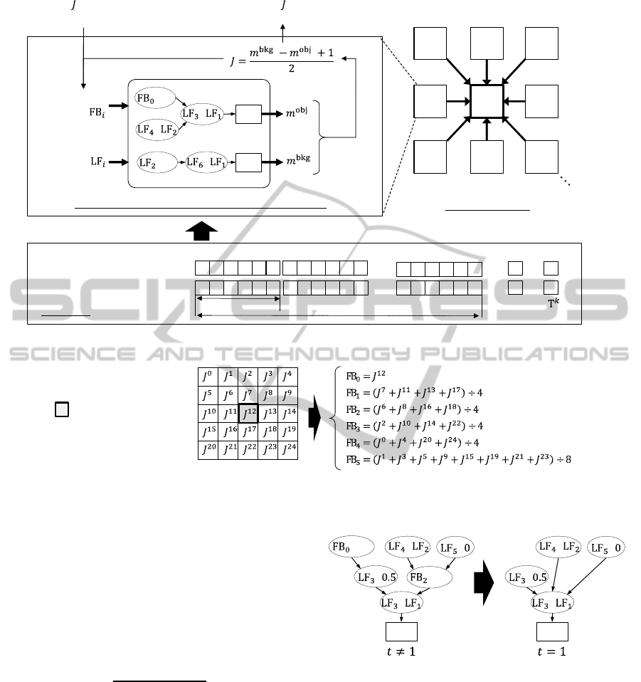
No. 0 No. 1 No. 2 No. 4 No. 5 No. 6 ConsequentNo. 3
5
: not appear in phenotype
(w = 0.5)
No. 0
(w = 0.1)
No. 1
No. 2
Class k
No. 4
No. 5
: If ( or ) and 0.5 then Class k
: If
0.5
then Class k
Phenotype
(a directed graph)
The condition in the
genotype doesn’t appear in
the consequent node
2 0 0 1 1 2 5 4 2 0 1 12 1 0 2 1 0 5 6 1 1 1 26 6 2 0 1 2 6 5 2 0 2 2 8 0 2 0 0 2
0.5
(w = 0.2)
: the consequent node
0.5
(w = 0.3)
To edge Condition type c w
ID
,
0
1
2
ID Condition
0
1
2
3
4
5
6
7
ID
0 0.1
1 0.2
2 0.3
ID
0 0.0
1 0.5
2 1.0
A subgraph having a path to
a consequent node indicates
an antecedent part of a rule.
Lookup
tables
Genotype (a numeric string)Rules for class k:
Figure 1: Example of genotype and phenotype representation of Fuzzy Oriented Classifier Evolution.
is one of Genetic Fuzzy Systems (GFSs) which de-
sign fuzzy rules by evolutionary algorithms (Herrera,
2008), and constructs fuzzy classification rules repre-
sented as directed graphs composed of nodes indicat-
ing fuzzy conditions. We expect FORCE constructs
fuzzy rules for segmentation efficiently because of the
compact and flexible graph representation. The sec-
ond feature is inspired by Cellular Neural Network
(CNN) (Chua and Yang, 1988). CNN consists of
a regular array of processing units called cells con-
nected with only their neighbor cells. Each cell com-
putes an output value iteratively considering output of
their neighbor cells besides local information. CNN
has showed good performance in image filtering in
spite of its simple structure. The proposed model
computes matching degree of pixels with object and
background iteratively with considering the matching
degree of neighbor pixels as CNN computes output
iteratively, to classify even the overlapped pixels cor-
rectly by considering their spatial relationship.
The remaining of this paper is organized in the fol-
lowing way. Section 2 reviews FORCE briefly, and
details of the proposed model are described in Sec-
tion 3. Experimental results are shown in Section 4.
Finally, in Section 5, we conclude this work.
2 FUZZY ORIENTED
CLASSIFIER EVOLUTION
Figure 1 illustrates an overview of FORCE. FORCE
represents fuzzy classification rules as a directed
graph composed of two types of nodes: condition
nodes and a consequent node that indicate conditions
and a predefined consequent of rules (classification
class) respectively. In the graph, series connections
of condition nodes are defined as AND operation of
the conditions and parallel connections are defined as
OR operation. A subgraph of the graph having a path
to a consequent node indicates an antecedent part of
a rule whose consequent part is defined by the con-
sequent node. Namely, one graph represents one rule
set for predefined class k such like that illustrated in
Figure 1. The rule set computes matching degree m
k
of data with class k. The graph is converted into a
numeric string (genotype) indicating connections and
parameters of each condition node and a consequent
node number, and developed by optimizing the string
by GA.
FORCE is expected to constructs fuzzy rules more
flexibly and efficiently than conventional GFSs based
on simple GA or Genetic Programming (Koza, 1992)
because of the compact graph representation. FORCE
has been applied to image classification tasks and
classification of benchmark data sets in comparison
with conventional methods, and constructed compact
and accurate classification rules (Otsuka and Nagao,
2012; Otsuka and Nagao, 2013).
3 CELLULAR FUZZY ORIENTED
CLASSIFIER EVOLUTION
3.1 Model Overview
An overview of CFORCE is described in Figure 2. In
CFORCE, a pair of graphs representing fuzzy classi-
fication rules for object (obj) and background (bkg)
class is defined as a processing unit, and the identical
units are allocated on each pixel over an input image.
The graphs of each unit output matching degree of
each pixel with obj and bkg class iteratively with con-
sidering local features (LFs) and feedback features
(FBs). LFs are such like standard statistics computed
from pixel values in a local window, and FBs indi-
cate magnitude of the matching degree of neighbor
pixels. After defined number of output iteration, each
pixel is classified as either obj or bkg associated with
the highest matching degree. In region segmentation,
spatial relationship between neighbor pixels is impor-
tant as well as local features. That is, neighbor pixels
tend to belong to be the same class. FBs are expected
to enable CFORCE to consider the relationship and
process complex object segmentation in which clus-
ters of pixels are overlapped.
EvolutionaryFuzzyRuleConstructionforIterativeObjectSegmentation
85
…
Local
features:
>
=0.1
=
obj
J
J
J J J
J
J J
…
>0.8
<
bkg
Feedback
features:
Input values from
neighbor units
Classification rules (graphs) for obj and bkg class
Output value to
neighbor units
No. 0 No. 1
2
0 0 1 1 2 2 1 0 2 0 1
3 0 4 1 2 2 5 5 1 2 1 0
...
...
25
3 0 2 1 1
28 8 3 2 0 2
No. U
10
21
2
5
Consequent
Node No.
genes for a node
genes for nodes
Genotype
A chromosome for obj class:
A chromosome for bkg class:
Unit
Unit Unit Unit
…
Unit Unit Unit
Unit Unit
…
…
Cellular FORCE
…
Figure 2: Overview of the proposed model.
J of neighbor pixels
is a target pixel for
which FBs are computed.
Figure 3: Feedback template: how to merge J values of neighbor units to six rotation invariant feedback features.
3.2 Feedback Features
FBs represent magnitude relation between matching
degree of neighbor pixels with obj and bkg class cal-
culated by neighbor graphs in the previous output. In
the t-th output, FBs of a pixel are calculated using
J
t−1
of neighbor pixels computed by the following
formula:
J
t−1
=
m
bkg
t−1
− m
obj
t−1
+ 1
2
, (1)
where m
obj
t−1
and m
bkg
t−1
are matching degree of a pixel
with obj and bkg class respectively computed by a
pair of graphs placed on the pixel in the (t-1)-th out-
put. J
t−1
indicates magnitude relation between m
obj
t−1
and m
bkg
t−1
. m
obj
t−1
, m
bkg
t−1
and J
t−1
are real numbers in
range [0, 1]. In this work, six types of 90 degrees ro-
tation invariant FBs are computed from neighbor J
t−1
in 5 × 5 pixels using a template illustrated in Figure
3. In the template, a target pixel is placed on the cen-
ter. FBs are used in condition nodes in the same way
as the other input features except when t = 1. When
Obj
= 0.1
< 0.3
>
=
>
=
Obj
>
=
>
=
Figure 4: Example of graphs when t 6= 1 and t = 1.
t = 1, FBs cannot be computed because m
bkg
0
and m
obj
0
are undefined. Therefore, condition nodes using FBs
are not used when t = 1. That is, they are simply ig-
nored such like that illustrated in Figure 4.
3.3 Graph Structure and Genotype
The structure of graphs is the same as that of FORCE
except that CFORCE employs FBs. In the graph, a
condition node represents a condition in a form of
“x
1
i
Operator V”, where x
1
i
is the i-th input feature,
ICAART2014-InternationalConferenceonAgentsandArtificialIntelligence
86
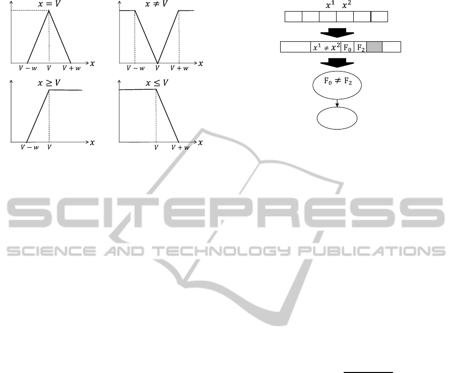
1
Matching degree
1
Matching degree
1
Matching degree
1
Matching degree
Figure 5: Membership functions used in this work.
Operator is a comparison operator ∈ {=, 6=, ≥, ≤},
and V is a constant c or input feature x
2
i
compared
with x
1
i
. In addition, each condition node has a pa-
rameter w for MFs. Figure 5 shows MFs correspond-
ing to each comparison operator used in the proposed
model. w determines slope and V (i.e., c or x
2
i
) deter-
mines position of MFs.
The genotype for a graph is a numeric string in
which genes deciding parameters for each condition
nodes (i.e., to edge, condition type, x
1
i
, x
2
i
, c and w),
a consequent node number, and an output iteration
number T line up. Table 1 shows the parameters for
graphs used in this work. Genes for condition nodes
are ID numbers associated with the parameters, and
each condition node is converted from the genes us-
ing lookup tables. Figure 6 illustrates an example of
converting genes to a condition node using Table 1.
Note that, genes for x
1
i
and x
2
i
indicate ID numbers
of input features including FBs. The length of the
genotype for a graph is fixed: 6U+ 2, where U is the
maximal number of nodes used for a graph. How-
ever, the number of nodes appearing in the phenotype
(active nodes) is variable because nodes not having a
path to a consequent node do not appear in the pheno-
type (inactive nodes). The graph is feedforward graph
as each node is allowed to connect to only nodes hav-
ing a larger node number than itself. The genotype of
CFORCE is a pair of the numeric string representing
graphs for obj and bkg class.
3.4 Object Segmentation Procedure
Using k ∈ {obj, bkg} and G
k
indicating a graph for
class k, the procedure of object segmentation by the
proposed model is described as follows:
1. t = 1.
2. Execute the following procedure for each class k.
2 1 0 2 0 1
(w = 0.2)
No. 2
To No.2 0.0 0.2
To
Cond.
c w
Figure 6: Example of converting genes to a condition node.
(a) If t is T
k
and less, G
k
executes (b) and (c).
(b) Compute matching degree µ
C
k
s
(X) between in-
put features X of each pixel with an antecedent
part C
k
s
defined by the s-th subgraph of G
k
by
the following fuzzy logic operators.
µ
A∩B
(X) = min{µ
A
(X), µ
B
(X)}, (2)
µ
A∪B
(X) = max{µ
A
(X), µ
B
(X)}, (3)
where A and B are arbitrary fuzzy conditions,
and µ is matching degree of X with the condi-
tions. Matching degree of X with a condition
of each condition node is computed by MF.
(c) Integrate µ
C
k
s
(X) into matching degree m
k
(X)
of X with class k on each pixel by the following
formula:
m
k
(X) =
Σ
S
k
s=1
µ
C
k
s
(X)
S
k
, (4)
where S
k
is the number of the subgraphs of G
k
.
More detailed process (b) and (c) are described
in Algorithm 1.
3. If t is less than max
T
obj
, T
bkg
, execute the fol-
lowing procedure.
(a) Compute J on each pixel by Equation 1.
(b) Compute FBs on each pixel by the template de-
scribed in Figure 3.
(c) t = t + 1, and go back to 2.
4. Classify each pixel as class k associated with the
highest m
k
(X).
3.5 Rule Evolution
The two graphs are optimized simultaneously using
GA employing simple two-point crossover and ran-
dom mutation as genetic operators. The fitness is de-
scribed by mainly two indicators of evaluation: “F”
and “IMP”. F is F-measure indicating classification
EvolutionaryFuzzyRuleConstructionforIterativeObjectSegmentation
87

Table 1: Parameters of CFORCE.
Parameters ID
0 1 2 3 4 5 6 7 8 9 10
Condition x
1
= x
2
x
1
6= x
2
x
1
≥ x
2
x
1
≤ x
2
x
1
= c x
1
6= c x
1
≥ c x
1
≤ c - - -
c 0.0 0.1 0.2 0.3 0.4 0.5 0.6 0.7 0.8 0.9 1.0
w
0.1 0.2 0.3 0.4 0.5 - - - - - -
T 1 2 3 4 5 - - - - - -
input : A pixel with input features X
An iteration number t
output: Matching degree m
k
of X with G
k
if t = 1 then
G
′
← G
k
without nodes using FBs;
else
G
′
← G
k
with nodes using FBs;
end
i ← 1;
n
i
← the i-th active node in G
′
;
while n
i
is not the consequent node do
from ← a set of nodes connected to n
i
;
if from is not empty then
µ
max
← max
n
j
∈ from
µ
n
j
;
else
µ
max
← 1;
end
µ
n
i
← min{µ
max
, MF
n
i
(X)};
i ← i+ 1;
n
i
← the i-th active node in G
′
;
end
from ← a set of nodes connected to n
i
;
if from is not empty then
S
k
← the number of nodes in from;
m
k
←
∑
n
j
∈ f rom
µ
n
j
S
k
;
/*
µ
n
j
= µ
C
k
s
*/
else
m
k
← 0;
end
Algorithm 1: How to compute m
k
(X) using G
k
.
accuracy, and IMP evaluates importance of obtained
rules. F is calculated by the following formula:
F =
2× N
correct
N+ N
detect
, (5)
where N is the number of obj pixels, N
correct
is the
number of obj pixels classified correctly, and N
detect
is the number of pixels classified as obj class. IMP is
the average product of Confidence (CD) and Support
(SP) of rules for each class, both represent importance
of rules. IMP is calculated by the following formula:
CD
k
=
Σ
N
k
n=1
m
k
X
k
n
Σ
N
l=1
m
k
(X
l
)
, (6)
SP
k
=
Σ
N
k
n=1
m
k
X
k
n
N
k
, (7)
IMP =
1
2
Σ
k∈{obj,bkg}
CD
k
· SP
k
, (8)
where X
k
n
indicates input features of the n-th pixel la-
beled as class k and N
k
is the number of pixels labeled
as class k. Finally, the fitness function is represented
as follows:
fitness = F× IMP+
ε
N
cond
, (9)
where N
cond
is the total number of condition nodes
used in graphs, and the last term evaluates compact-
ness of rules. ε is a small weight value (ε = 0.001 in
this paper).
4 EXPERIMENTS
4.1 Overview of Experiments
We tested CFORCE using three different object seg-
mentation tasks to evaluate performance of the model.
• Crack extraction (grayscale)
This task requires extracting cracks in concrete
wall from images containing cracks and lines not
cracks. Figure 7 shows training images, and
Figure 8 shows test images not used in training
and used to examine the performance of obtained
rules. The images are 128× 128 pixels.
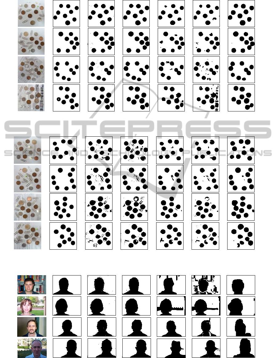
• Coin extraction (color)
This task requires extracting several coins from
images containing coins and other objects. Fig-
ure 9 and Figure 10 show training and test images
respectively. The images are 128× 128 pixels.
• Human extraction (color)
This task requires extracting human’s busts from
images in varied light conditions and various
ICAART2014-InternationalConferenceonAgentsandArtificialIntelligence
88

backgrounds. Figure 11 and Figure 12 show
parts of training and test images respectively. We
selected 10 images for training and 20 images
for test from the MSRC Object Category Im-
age Database v2
1
. Originally these images are
320 × 213 pixels and labeled roughly. In this ex-
periment, we reduced them to 100× 67 pixels and
labeled them precisely.
For comparison, we also applied four compara-
tive methods to the same tasks: the original FORCE,
Support Vector Machine (SVM) (Vapnik, 2000), C4.5
(Quinlan, 1993), and a graph cuts based segmentation
method (GC). GC is a method based on Interactive
Graph Cuts (Boykov and Jolly, 2001) which divide an
image into object and backgroundregionsusing graph
cuts to find globally optimal segmentation. Interac-
tive Graph Cuts use seeds marked pixels as object or
background by a user to provide hard constraints for
segmentation and to compute histogram for object or
background intensity distributions. GC does not use
seeds and computes the histogram from pixel values
of training images.
4.2 Experimental Settings
Input features used in the experiments are shown in
Table 2. The features were standard statistics com-
puted from pixel values in a local window of 5 × 5
pixel size, six FBs, and six rotation invariant pixel
values I
i
computed from neighbor pixel values us-
ing the same template as FBs. For color images, we
used L*a*b* color space, and the input features ex-
cept FBs are computed from each color component.
The “Groups” indicates the groups of input features
allowed to be compared each other in CFORCE. A
condition comparing input features x
1
i
and x
2
i
in dif-
ferent groups is changed to a condition comparing an
input feature x
1
i
and a constant c.
CFORCE and FORCE were tested six times with
different random seed in each experiment using the
following parameters: the number of generations was
10000, the population size was 50, the crossover rate
was 0.7, and the mutation rate was 0.02. Minimal
Generation Gap model [15] was used as a genera-
tion alternation model, and the number of children
was 30. The maximal number of nodes U for each
graph was 60. These parameters are based on the pre-
vious work. SVM and C4.5 were run using WEKA
(Hall et al., 2009). SVM employed RBF kernel,
and γ of the RBF kernel and the complexity parame-
ter C were selected from {2
n
|n = −7, −6, .., 1, 2} and
{2
n
|n = −2, −1, .., 6, 7} respectively by grid search in
1
http://research.microsoft.com/en-
us/projects/ObjectClassRecognition/
Table 2: Input features used in this work.
Groups Features
0 Max, Min, Mean, Median,
First quartile, Third quartile,
Six rotation invariant pixel values: I
i
1 Standard deviation
2 Range
3 Averaged edge magnitude
4 Skewness
5 Kurtosis
6 Six feedback features: FB
i
each task. The minNumObj and confidenceFactor
of C4.5 were also selected from {0, 1, 2, 3, 4, 5} and
{0.1, 0.2, 0.3, 0.4, 0.5} respectively by grid search.
For GC, we selected BIN# of histogram from
{16, 32, 64, 128, 256}, σ of boundarypenalty function
from {0.1, 0.3, 0.5, 0.7, 0.9, 1.1, 1.3, 1.5} and λ a pa-
rameter for edge weights from {1, 2, 4, 8, 16, 32, 64}
to maximize F-measure for training images in each
task.
4.3 Results and Discussion
Accuracy results (F-measure) of the experiments are
summarized in Table 3. The values in parentheses
of FORCE and CFORCE are averaged results over
six runs, and the other values of them are results of
the elitist rules obtained in training. SVM and C4.5
processed the training images better than CFORCE in
coin and human extraction, but for the test images, the
elitist rules of CFORCE showed the most accurate re-
sults in all experiments. That is, CFORCE prevented
rules from overfitting the training images better than
SVM and C4.5. GC showed better results for the test
images in the coin and human extraction than SVM,
C4.5 and FORCE, although it hardly processed crack
extraction because the histogram based on gray level
is too simple to represent differences between cracks
and background.
The result images processed by each method are
shown in Figure 7-12. The feature of processing by
CFORCE is that extracted regions tend to be united
with little noises (small misclassified regions), al-
though boundaries between regions are likely impre-
cise a little. We consider this feature is caused by
FBs because results of FORCE without FBs do not
show such features, and some results of GC consid-
ering relationship between pixels have similarity to
those of CFORCE. SVM and C4.5 produced good
results with precise boundaries for the training im-
ages, but the test results of them have more noises
than those of CFORCE. Figure 13 illustrates an exam-
EvolutionaryFuzzyRuleConstructionforIterativeObjectSegmentation
89
Table 3: Accuracy results (F-measure) of each method.
SVM C4.5 GC FORCE CFORCE
Best (Avg.) Best (Avg.)
Crack Training 0.910 0.930 0.061 0.788 (0.764) 0.930 (0.891)
Test 0.665 0.567 0.056 0.712 (0.718) 0.827 (0.829)
Coin Training 1.000 0.997 0.938 0.915 (0.896) 0.997 (0.989)
Test 0.936 0.928 0.958 0.931 (0.915) 0.968 (0.972)
Human Training 1.000 0.998 0.851 0.843 (0.826) 0.904 (0.855)
Test 0.755 0.720 0.759 0.718 (0.714) 0.794 (0.744)
Avg. Training 0.970 0.975 0.616 0.849 (0.829) 0.944 (0.912)
Test 0.785 0.739 0.591 0.787 (0.782) 0.863 (0.848)
(a) Training images (c) C4.5 (d) SVM (f) FORCE (g) CFORCE(e) GC(b) Ground truth
Figure 7: Training images and results of each method in crack extraction.
(a) Test images (c) C4.5 (d) SVM (f) FORCE (g) CFORCE(e) GC(b) Ground truth
Figure 8: Test images and results of each method in crack extraction.
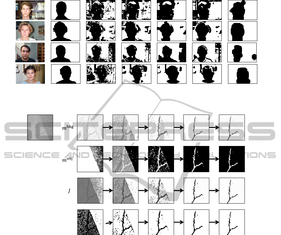
ple of crack extraction by the elitist rule developed by
CFORCE. The brighter pixels indicate higher values
in each image. We can see that each graph intensifies
m
k
of pixels belonging to class k gradually by consid-
ering their neighbor J values (FBs), and decreases the
number of misclassified pixels which are hard to be
classified by only local features. These visualized re-
sults show that iterative process with FBs worked effi-
ciently for segmentation. Note that, in CFORCE, the
number of output iteration is decided by a gene, and
does not consider convergence of processing. There-
fore, if output process iterates over defined times, un-
desirable results can occur, i.e., misclassified regions
can increase. The relationship between the iteration
ICAART2014-InternationalConferenceonAgentsandArtificialIntelligence
90
(a) Training images (c) C4.5 (d) SVM (f) FORCE (g) CFORCE(e) GC(b) Ground truth
Figure 9: Training images and results of each method in coin extraction.
(a) Test images (c) C4.5 (d) SVM (f) FORCE (g) CFORCE(e) GC(b) Ground truth
Figure 10: Test images and results of each method in coin extraction.
(a) Training images (c) C4.5 (d) SVM (f) FORCE (g) CFORCE(e) GC(b) Ground truth
Figure 11: Examples of training images and results of each method in human extraction.
EvolutionaryFuzzyRuleConstructionforIterativeObjectSegmentation
91
(a) Test images (c) C4.5 (d) SVM (f) FORCE (g) CFORCE(e) GC(b) Ground truth
Figure 12: Examples of test images and results of each method in human extraction.
The 1st output The 2nd output The 3rd output The 4th output The 5th outputThe input image
Result
Figure 13: Example of output transition of CFORCE obtained in crack extraction.
times and convergence should be investigated in fu-
ture works.
5 CONCLUSIONS
In this paper, CFORCE the novel method to construct
fuzzy classification rules for image segmentation was
presented. The algorithm has mainly two features: 1)
designing fuzzy rules for object and background clas-
sification using FORCE which develops fuzzy rules
represented as directed graphs automatically by GA,
and 2) performing iterative segmentation with consid-
ering spatial relationship between pixels. In natural
image segmentation, many pixels are overlapped be-
tween different clusters. Therefore, considering the
spatial relationship besides local features is important
to classify the overlapped pixels correctly. The pro-
posed model constructs fuzzy classification rules in
which spatial features considering the spatial relation-
ship are incorporated, and extracts object region by
the rules in iterativeprocess even if the clusters of pix-
els are overlapped. The experimental results showed
that CFORCE constructed fuzzy rules for three differ-
ent image segmentation successfully.
In this work, the number of output iteration was
decided by a gene, and it did not relate to convergence
of segmentation process. Investigating relationship
between the iteration times and convergence is one of
our future works. Additionally, we also plan to extend
the model to multi-class segmentation.
ACKNOWLEDGEMENTS
This work was supported by JSPS KAKENHI Grant
Number 25·2243.
ICAART2014-InternationalConferenceonAgentsandArtificialIntelligence
92

REFERENCES
Beevi, Z. and Sathik, M. (2012). A robust segmentation
approach for noisy medical images using fuzzy clus-
tering with spatial probability. methods, 29(37):38.
Borji, A. and Hamidi, M. (2007). Evolving a fuzzy rule-
base for image segmentation. International Journal
of Intelligent Systems and Technologies, 28:178–183.
Boykov, Y. Y. and Jolly, M.-P. (2001). Interactive graph
cuts for optimal boundary & region segmentation of
objects in nd images. Computer Vision, 2001. ICCV
2001. Proceedings. Eighth IEEE International Con-
ference on, 1:105–112.
Chua, L. O. and Yang, L. (1988). Cellular neural networks:
Applications. Circuits and Systems, IEEE Transac-
tions on, 35(10):1273–1290.
Hall, M., Frank, E., Holmes, G., Pfahringer, B., Reute-
mann, P., and Witten, I. H. (2009). The weka data
mining software: an update. SIGKDD Explor. Newsl.,
11(1):10–18.
Herrera, F. (2008). Genetic fuzzy systems: taxonomy, cur-
rent research trends and prospects. Evolutionary In-
telligence, 1(1):27–46.
Karmakar, G. C. and Dooley, L. S. (2002). A generic fuzzy
rule based image segmentation algorithm. Pattern
Recognition Letters, 23(10):1215–1227.
Karmakar, G. C., Dooley, L. S., and Rahman, S. (2000). A
survey of fuzzy rule-based image segmentation tech-
niques.
Koza, J. R. (1992). Genetic programming: on the program-
ming of computers by means of natural selection. MIT
Press, Cambridge, MA, USA.
Lai, Y. and Lin, P. (2008). Effective segmentation for den-
tal x-ray images using texture-based fuzzy inference
system. pages 936–947.
Otsuka, J. and Nagao, T. (2012). Flexible design of im-
age classification rules using extended fuzzy oriented
classifier evolution. In Soft Computing and Intelligent
Systems (SCIS) and 13th International Symposium on
Advanced Intelligent Systems (ISIS), 2012 Joint 6th
International Conference on, pages 1595–1600.
Otsuka, J. and Nagao, T. (2013). Automatic construction
of fuzzy classification rules for pattern classification
using fuzzy oriented classifier evolution. The IEICE
transactions on information and systems, 96(1):158–
167 (in Japanese).
Quinlan, J. R. (1993). C4.5: programs for machine learn-
ing. Morgan Kaufmann Publishers Inc., San Fran-
cisco, CA, USA.
Stavrakoudis, D., Theocharis, J., and Zalidis, G. (2011). A
boosted genetic fuzzy classifier for land cover classi-
fication of remote sensing imagery. ISPRS Journal
of Photogrammetry and Remote Sensing, 66(4):529–
544.
Vapnik, V. (2000). The nature of statistical learning theory.
springer.
EvolutionaryFuzzyRuleConstructionforIterativeObjectSegmentation
93
