
Control of the p53 Protein - mdm2 Inhibitor System
using Nonlinear Kalman Filtering
Gerasimos G. Rigatos
1
and Efthymia G. Rigatou
2
1
Unit of Industrial Automation, Industrial Systems Institute, Stadiou str., 26504 Rion Patras, Greece
2
Dept. of Paediatric Haematology-Oncology, Athens Children Hospital ”Aghia Sofia”, 11527, Athens, Greece
Keywords:
p53 Protein Synthesis, mdm2 Inhibitor, Nonlinear Feedback Control, Differential Flatness Theory, Derivative-
free Nonlinear Kalman Filter.
Abstract:
A nonlinear feedback control scheme for the p53 protein - mdm2 inhibitor system is developed with the use of
differential flatness theory and of nonlinear Kalman Filtering. It is shown that by applying differential flatness
theory the protein synthesis model can be transformed into the canonical form. This enables the design of a
feedback control law that maintains the concentration of the p53 protein at the desirable levels. To estimate the
non-measurable elements of the state vector describing the p53-mdm2 system dynamics and to compensate
for modeling uncertainties and external disturbances that affect the p53-mdm2 system, the nonlinear Kalman
Filter is re-designed as a disturbance observer. The proposed nonlinear feedback control and perturbations
compensation method for the p53-mdm2 system can result in more efficient chemotherapy schemes where the
infusion of medication will be better administered.
1 INTRODUCTION
The P53 protein has been identified as a key factor
in the abatement of tumors since it enhances cell-
cycle arrest and apoptosis. The concentration of the
P53 protein in the cytoplasm is primarily controlled
by another protein, known as inhibitor protein mdm2,
within a feedback loop. When the concentration of
the MDM2 protein increases, the concentration of the
P53 protein is reduced (downregulation). The MDM2
protein binds ubiquitin molecules to P53 which re-
sult to the disintegration of the P53 protein. On
the other side, the increase of the concentration of
P53 enhances the transcription procedure of mdm2
and consequently the produced MDM2 protein will
downregulate P53. In this manner the p53-mdm2
feedback loop converges to an equilibrium (Lillacci
et al., 2006),(Qi et al., 2008),(Wagner et al., 2005).
There are chemotherapy drugs that work by binding
the MDM2 protein and consequently by preventing
the MDM2 protein from disintegrating the P53 pro-
tein (ubiquitination) (Elias et al., 2013),(Abou-Jaoud´e
et al., 2010). This is a promising approach to the treat-
ment of cancer. It is based on the infusion of MDM2
antagonists which are called Nutlins. By deactivating
MDM2 these drugs restore the levels of concentra-
tion of the P53 protein and consequently contribute
to the fighting against cancel cells (Jahoor Alam et
al., 2012),(Pierce and Findley, 2010),(Leenders and
Tuszynski, 2013).
In this paper it is shown that it is possible to con-
trol the levels of the concentration of the P53 protein
through nonlinear feedback control, where the con-
trol input is the infusion rate of the chemotherapy
drug. Previous results on nonlinear feedback con-
trol of biological oscillators and on control of pro-
tein synthesis processes can be found in (Rigatos,
2013),(Rigatos and Rigatou, 2013). The pharma-
cokinetics - pharmacodynamics model of the P53
protein is described by a complicated set of non-
linear differential equations. It is shown that with
the use of differential flatness theory it is possi-
ble to transform this complicated model into the
canonical Brunovsky form (Rudolph, 2003),(Sira-
Ramirez and Agrawal, 2004),(L´evine, 2011),(Fliess
and Mounier, 1999),(Rouchon, 2005),(Martin and
Rouchon, 1999),(Bououden et al., 2011), (Laroche
et al., 2007). In this latter form a single-input sin-
gle output description between the output (P53 pro-
tein) and the input (drug’s infusion rate) is obtained
and this facilitates the design of a feedback control
and state estimation scheme that can make the P53
protein concentration convergeto the desirable levels.
Moreover, disturbances estimation and compensation
209
G. Rigatos G. and G. Rigatou E..
Control of the p53 Protein - mdm2 Inhibitor System using Nonlinear Kalman Filtering.
DOI: 10.5220/0004866702090214
In Proceedings of the International Conference on Bioinformatics Models, Methods and Algorithms (BIOINFORMATICS-2014), pages 209-214
ISBN: 978-989-758-012-3
Copyright
c
2014 SCITEPRESS (Science and Technology Publications, Lda.)
is performed with the use of nonlinear Kalman Filter-
ing.
2 DYNAMIC MODEL OF THE p53
PROTEIN - mdm2 INHIBITOR
SYSTEM
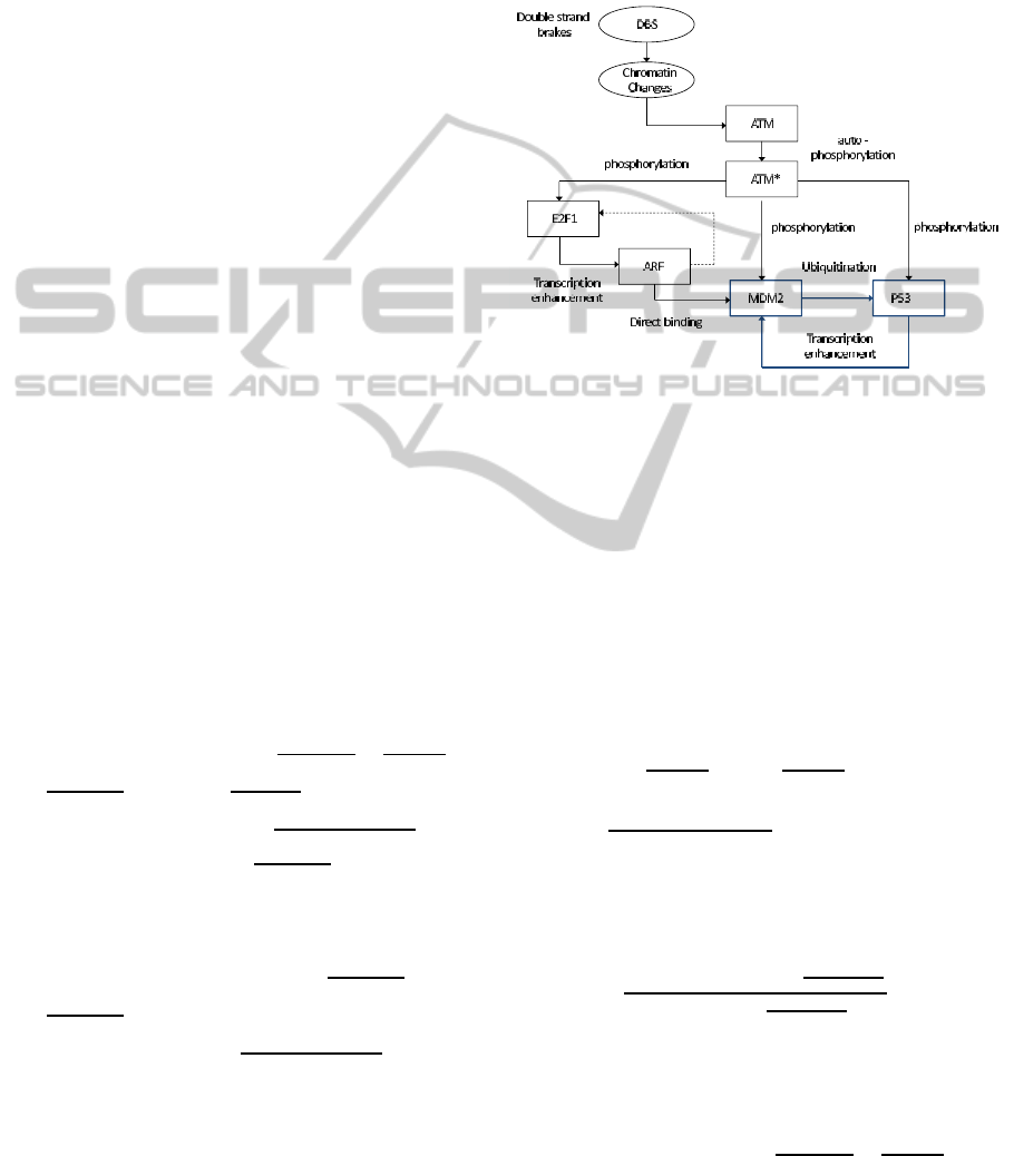
The meaning of the variables that appear in the p53
protein - mdm2 inhibitor dynamical system (see Fig.
1) is as follows (Lillacci et al., 2006), (Qi et al., 2008),
(Elias et al., 2013), (Jahoor Alam et al., 2012): p53:
mRNA concentration of the p53 gene after transcrip-
tion, P53: concentration of the P53 protein in the cy-
toplasm after translation, P53
∗
: active form of the P53
protein that is produced after phosphorylation of P53,
mdm2: mRNA concentration of the inhibitor pro-
tein mdm2 after transcription, MDM2: concentration
of the MDM2 protein in the cytoplasm after transla-
tion, N: concentration of the chemotherapeutic drug,
ATM: a protein that identifies the transcription of p53
and contributes to the phosphorylation of the P53 pro-
tein, ATM
∗
: concentration of the active form of the
ATM protein. It contributes both to the phosphory-
lation of protein P53 and of protein MDM2, e2f1:
mRNA concentration of the gene e2f1 after transcrip-
tion, E2F1: concentration of the protein E2F1 after
translation, E2F1
∗
: active form of the E2F1 protein,
ar f: mRNA concentration of the gene ar f after tran-
scription, ARF: concentration of the ARF protein af-
ter translation. The associated state-space model is
(Lillacci et al., 2006):
˙x
1
= λ
p53
− µ
p53
x
1
˙x
2
= a
p53
x
1
− µ
53
x
2
− v
p53
x
3
−
K
1
ATM
∗
x
2
K
M
1
+x
2
−
K
cat
x
5
x
2
aK
13
+x
2
˙x
3
=
K
1
ATM
∗
x
2
K
M
1
+x
2
− v
p53
x
3
−
K
c
at
∗
x
5
x
3
aK
13
+x
3
˙x
4
= λ
mdm2
− µ
mdm2
x
4
+ φ
mdm2
x
3
(t−r
1
)
n
1
x
2
(0)
n
1
+x
3
(t−r
1
)
n
1
˙x
5
= a
MDM2
x
4
− µ
MDM2
x
5
−
K
2
ATM
∗
x
5
K
M
2
+x
5
−
−K
4
x
11
x
5
− K
6
x
6
x
5
˙x
6
= λ
N
− µ
N
x
6
− K
6
x
6
x
5
˙x
7
= λ
e2f1
− µ
e2f1
x
7
˙x
8
= a
E2F1
x
7
− µ
E2F1
x
8
+ v
E2F1
x
9
−
K
2
ATM
∗
x
8
K
M
3
+x
8
˙x
9
=
K
3
ATM
∗
x
8
K
M
3
+x
8
− v
E2F1
x
9
− K
5
x
11
x
9
˙x
10
= λ
ar f
− µ
ar f
x
10
+ φ
ar f
x
9
(t−r
2
)
n
2
x
8
(0)
n
2
+x
9
(t−r
2
)
n
2
˙x
11
= a
ARF
x
10
− µ
ARF
x
11
− K
4
x
11
x
5
− K
5
x
11
x
9
(1)
where the state variables for the dynamic model of the
p53 protein - mdm2 inhibitor system of Eq. (1) are de-
fined as: x
1
= p53, x
2
= P53, x
3
= P53
∗
, x
4
= mdm2,
x
5
= MDM2, x
6
= N, x
7
= e2f1, x
8
= E2F1, x
9
=
E2F1
∗
, x
10
= ar f and x
11
= ARF. In matrix form,
the state-space description of the system becomes
˙x = f(x) + g(x)u
(2)
where u = λ
N
is the control input (drug infusion rate),
and f(x)∈R
11×1
, g(x)∈R
11×1
are vector fields.
Figure 1: Feedback control loop of the p53 protein - mdm2
inhibitor system.
3 FLATNESS-BASED CONTROL
OF THE p53 PROTEIN SYSTEM
First, it will be shown that the considered model of
the p53 protein - mdm2 inhibitor system is a differ-
entially flat one. The following flat output is defined
y = [p
∗
53
, N, E2F1
∗
, ARF] or y = [x
1
, x
6
, x
9
, x
11
]. Thus
one has y = [y
1
, y
2
, y
3
, y
4
]
T
. From the sixth row of Eq.
(1) and by solving with respect to x
5
one obtains
x
5
=
˙x
6
+µ
N
x
6
−K
6
x
6
⇒x
5
=
˙y
2
+µ
N
y
2
−K
6
y
2
⇒
x
5
=
[0 1 0 0] ˙y+µ
N
[0 1 0 0]y
−K
6
[0 1 0 0]y
⇒x
5
= f
5
(y, ˙y)
(3)
From the third row of Eq. (1) and by solving with
respect to x
2
one obtains
x
2
=
K
M
1
˙y
1
−v
p53
K
M
1
y
1
+K
M
1
K
∗
cat
f
5
(y, ˙y)y
1
aK
13
+y
1
K
1
ATM
∗
+v
p53
y
1
+
K
∗
cat
f
5
(y, ˙y)y
1
aK
13
+y
1
− ˙y
1
⇒
x
2
= f
2
(y, ˙y)
(4)
Equivalently, the second row of Eq. (1) is solved with
respect to x
1
. This gives
x
1
= ˙x
2
+ µ
p53
x
2
+ v
p53
x
3
+
K
1
ATM
∗
x
2
K
M
1
+x
2
−
K
cat
x
2
x
5
aK
13
+x
2
⇒
x
1
= f
1
(y, ˙y)
(5)
BIOINFORMATICS2014-InternationalConferenceonBioinformaticsModels,MethodsandAlgorithms
210

The fifth row of Eq. (1) is solved with respect to x
4
x
4
=
˙x
5
+µ
MDM2
x
5
+
K
2
ATM
∗
x
5
K
M
2
+X
5
+K
4
x
11
x
5
+K
6
x
6
x
5
a
MDM2
⇒
x
4
= f
4
(y, ˙y)
(6)
The ninth row of Eq. (1) is solved with respect to x
8
K
M
3
˙x
9
+ ˙x
9
x
8
= K
3
ATM
∗
x
8
− v
E2F1
K
M
3
x
9
−
−v
E2F1
x
8
x
9
− K
5
K
M
3
x
11
x
9
− K
5
x
11
x
9
x
8
⇒
x
8
=
K
M
3
˙x
9
+v
E2F1
K
M
3
x
3
+K
5
K
M
3
x
11
x
9
K
3
ATM
∗
− ˙x
9
−v
E2F1
x
9
−K
9
x
11
x
9
⇒
x
8
= f
8
(y, ˙y)
(7)
The eighth row of Eq. (1) is solved with respect to x
7
x
7
=
˙x
8
+µ
E2F1
x
8
−v
E2F1
x
9
+
K
2
ATM
∗
x
8
K
M
3
+x
8
a
E2F1
⇒
x
7
= f
7
(y, ˙y)
(8)
The eleventh row of Eq. (1) is solved for x
10
x
10
=
˙x
11
+µ
ARF
x
11
+K
4
x
11
x
5
+K
5
x
11
x
9
a
ARF
⇒
x
10
= f
10
(y, ˙y)
(9)
Moreover, from the sixth row of Eq. (1) and using
that x
5
= f
5
(y, ˙y) and x
6
= y
2
one obtains about the
control input u = λ
N
u = λ
N
= ˙x
6
+ µ
N
x
6
+ K
6
x
6
x
5
⇒
λ
N
= f
u
(y, ˙y)
(10)
Thus one has that all state variables and the control
input of the p53 protein - mdm2 inhibitor system are
functions of the flat output y and of its derivatives.
Consequently, the dynamical system of P53 protein
is a differentially flat one.
Next, it will be shown that using the differentially
flat description of the p53 protein - mdm2 inhibitor
system it is possible to transform it to the canonical
Brunovsky form. It holds that y
1
= x
3
therefore
˙y
1
= ˙x
3
⇒ ˙y
1
=
K
1
ATM
∗
x
2
K
M
1
+x
2
− v
P53
x
3
−
K
∗
cat
x
5
x
3
aK
13
+x
3
(11)
Consequently, the second derivative of y
1
is
¨y
1
=
(K
1
ATM
∗
˙x
2
)(K
M
1
+x
2
)−(K
1
ATM
∗
x
2
) ˙x
2
(K
M
1
+x
2
)
2
− v
p53
˙x
3
−
−K
∗
cat
( ˙x
5
x
3
+x
5
˙x
3
)(aK
13
+x
3
)−(K
∗
cat
x
5
x
3
) ˙x
3
(aK
13
+x
3
)
2
(12)
After intermediate operations one obtains
¨y
1
=
K
1
ATM
∗
K
M
1
(K
M
1
+x
2
)
2
˙x
2
− v
p53
˙x
3
−
K
∗
cat
aK
13
x
5
˙x
3
(aK
13
+x
3
)
2
−
K
∗
cat
x
3
(aK
13
+x
3
)
˙x
5
(13)
and after substituting ˙x
3
and ˙x
5
one gets
¨y
1
=
K
1
ATM
∗
K
M
1
(K
M
1
+x
2
)
2
[a
p53
x
1
− µ
p53
x
2
−
v
p53
x
3
−
K
1
ATM
∗
x
2
K
M
1
+x
2
−
K
cat
x
5
x
2
(aK
13
+x
2
)
2
] − [v
p53
+
K
∗
cat
aK
13
x
5
(aK
13
+x
3
)
2
]·[
K
1
ATM
∗
x
2
K
M
1
+x
2
− v
p53
x
3
−
K
∗
cat
x
5
x
3
(aK
13
+x
3
)
] −
K
∗
cat
x
3
(aK
13
+x
3
)
[a
MDM2
x
4
− µ
MDM2
x
5
−
K
2
ATM
∗
x
5
K
M
2
+x
5
−
K
4
x
11
x
5
− K
6
x
6
x
5
].
By differentiating once more with respect to time one
obtains y
(3)
1
= f(y, ˙y) + g(y, ˙y)u, where the control
input u = λ
N
is the input rate of the chemotherapy
drug, while functions f(y, ˙y) and g(y, ˙y) are:
f(y, ˙y) = −
2(K
M
1
+x
2
) ˙x
2
K
1
ATMK
M
1
(K
M
1
+x
2
)
4
[a
p53
˙x
1
− µ
p53
˙x
2
−
v
p53
˙x
3
−
K
1
ATM
∗
x
2
K
M
1
+x
2
−
K
cat
x
5
x
2
aK
13
+x
2
] +
K
1
ATM
∗
K
M
1
(K
M
1
+x
2
)
2
[a
p53
˙x
1
−
µ
p53
˙x
2
− v
p53
˙x
3
−
K
1
ATM ˙x
2
(K
M
1
+x
2
)−K
1
ATM
∗
˙x
2
(K
M
1
+x
2
)
2
−
K
cat
( ˙x
5
x
2
+x
5
˙x
2
)(aK
13
+x
2
)−K
cat
x
5
x
2
˙x
2
(aK
13
+x
2
)
2
] −
−K
∗
cat
aK
13
˙x
5
(aK
13
+x
3
)
2
−K
∗
cat
aK
13
x
5
2(aK
13
+x
3
) ˙x
3
(aK
13
+x
3
)
4
·[
K
1
ATM
∗
x
2
K
M
1
+x
2
−
v
p53
x
3
−
K
c
at
∗
x
5
x
3
aK
13
+x
3
] − [v
p53
+
K
∗
cat
aK
13
x
5
(aK
13
+x
3
)
2
]·[
K
1
ATM
∗
˙x
2
(K
M
1
+x
2
)−K
1
ATM
∗
x
2
˙x
2
K
M
1
+x
2
2
−
v
p53
˙x
3
−
K
∗
cat
( ˙x
5
x
3
+x
5
˙x
3
)(aK
13
+x
3
)−K
∗
cat
x
5
x
3
(aK
13
+x
3
)
(aK
13
+x
3
)
2
] −
K
∗
cat
˙x
3
(aK
13
+x
3
)−K
c
at
∗
x
3
˙x
3
(aK
13
+x
3
)
2
·[a
MDM2
x
4
−
µ
MDM2
x
5
−
K
2
ATM
∗
x
5
K
M
2
+x
5
− K
4
x
11
x
5
−
K
6
x
6
x
5
] −
K
∗
cat
x
3
(aK
13
+x
3
)
·[a
MDM2
˙x
4
] − µ
MDM2
˙x
5
−
K
2
ATM
∗
x
5
−K
M
2
ATM
∗
x
5
˙x
5
K
M
2
+x
5
2
− K
4
( ˙x
11
x
5
+ x
11
˙x
5
) −
K
6
x
6
˙x
5
] −
K
∗
cat
x
3
(aK
13
+x
3
)
[−µ
N
x
6
− K
6
x
6
x
5
](−K
6
x
5
)
and g(y, ˙y) = −
K
∗
cat
x
3
aK
13
+x
3
(−K
6
x
5
). By defining the new
control input v = f(y, ˙y) + g(y, ˙y)u, the dynamics of
the active P53 protein can be written in the form
y
(3)
= f(y, ˙y) + g(y, ˙y)u⇒y
(3)
= v
(14)
A suitable feedback control law for the system of Eq.
(14) is given by
v = y
(3)
d
− k
1
( ¨y− ¨y
d
) − k
2
( ˙y− ˙y
d
) − k
3
(y− y
d
)
(15)
where the gains k
1
, k
2
and k
3
are chosen such that
the characteristic polynomial of the closed-loop sys-
tem to be a Hurwitz-stable one. The dynamics of the
tracking error is e = y− y
d
= P53
∗
− P53
∗
d
is given by
e
(3)
+ k
1
¨e + k
2
˙e + k
3
e = 0, which finally results into
lim
t→∞
e(t) = 0. The control input that actually ap-
Controlofthep53Protein-mdm2InhibitorSystemusingNonlinearKalmanFiltering
211

plied to the p53 protein - mdm2 inhibitor system is
computed from u = g(y, ˙y)
−1
[v− f(y, ˙y)]
4 DISTURBANCES
COMPENSATION USING
NONLINEAR KALMAN
FILTERING
To apply the feedback control law of Eq. (15) to the
system of the p53 protein synthesis it is possible to
use measurements of the concentration of the active
P53
∗
protein concentration at the cytoplasm, however
the derivatives of P53
∗
with respect to time are miss-
ing. Moreover, the p53-mdm2 dynamic model is sub-
jected to modeling uncertainties and external distur-
bances which are denoted by the aggregate term
˜
d in
the following equation:
y
(3)
= f(y, ˙y) + g(y, ˙y)u+
˜
d
(16)
The dynamics of the additive disturbance term
˜
d can
be equivalently represented through knowledge of the
associated n-th order derivative. Here, without loss
of generality it is considered that n = 3 thus one
has
˜
d
(3)
= f
d
. Next, the system’s state vector is ex-
tended so as to include the disturbance term’s dynam-
ics. The extended state vector contains the following
state variables: z
1
= y, z
2
= ˙y, z
3
= ¨y, z
4
=
˜
d, z
5
=
˙
˜
d
and z
6
=
¨
˜
d. Then the dynamics of the p53 protein -
mdm2 inhibitor system, including the modeling un-
certainty and external disturbances terms is written in
the following canonical Brunovsky form ˙z = Az+ Bv
and z
m
= Cz, or equivalently
˙z
1
˙z
2
˙z
3
˙z
4
˙z
5
˙z
6
=
0 1 0 0 0 0
0 0 1 0 0 0
0 0 0 1 0 0
0 0 0 0 1 0
0 0 0 0 0 1
0 0 0 0 0 0
z
1
z
2
z
3
z
4
z
5
z
6
+
0 0
0 0
1 0
0 0
0 0
0 1
v
f
d
(17)
with measurement equation given by
z
m
=
1 0 0 0 0 0
z (18)
For the dynamics of the p53 protein - mdm2 inhibitor
that is described by Eq. (17) and Eq. (18) it is pos-
sible to perform simultaneous estimation of the non-
measurable state variables as well as of the exter-
nal disturbances using the Kalman Filter recursion.
The application of Kalman Filtering on the linearized
equivalent of the system and the use of an inverse
transformation based on the expression of the initial
state variables as functions of the flat output (see Eq.
(3) to Eq. (7)) enables also to obtain estimates for the
state variables of the initial nonlinear dynamical sys-
tem. This recursive estimation and inverse transfor-
mation procedure constitutes the Derivative-free non-
linear Kalman Filter. The disturbance estimator is
˙
ˆz = A
o
ˆz+ B
o
u+ K(z
m
− ˆz
m
)
ˆz
m
= C
o
ˆz
(19)
where A
o
= A, C
o
= C and
B
T
o
=
0 0 1 0 0 0
0 0 0 0 0 0
(20)
In the design of the associated disturbances’ estimator
one has the dynamics defined in Eq. (19), where
K∈R
6×1
is the state estimator’s gain and matrices A
o
,
B
o
and C
o
have been defined in Eq. (17) to Eq. (18).
The discrete-time equivalents of matrices A
o
, B
o
and
C
o
are denoted as
˜
A
d
,
˜
B
d
and
˜
C
d
respectively, and
are computed with the use of common discretization
methods (Rigatos, 2011),(Rigatos and Zhang, 2009).
Next, a Derivative-free nonlinear Kalman Filter can
be designed for the aforementioned representation of
the system dynamics (Rigatos, 2011). The associated
Kalman Filter-based disturbance estimator is given
by the recursion (Rigatos and Tzafestas, 2007),(Bas-
sevile and Nikiforov, 1993),(Rigatos and Zhang,
2009)
measurement update:
K(k) = P
−
(k)
˜
C
T
d
[
˜
C
d
·P
−
(k)
˜
C
T
d
+ R]
−1
ˆz(k) = ˆz
−
(k) + K(k)[
˜
C
d
z(k) −
˜
C
d
ˆz
−
(k)]
P(k) = P
−
(k) − K(k)
˜
C
d
P
−
(k)
(21)
time update:
P
−
(k+ 1) =
˜
A
d
(k)P(k)
˜
A
T
d
(k) + Q(k)
ˆz
−
(k+ 1) =
˜
A
d
(k)ˆz(k) +
˜
B
d
(k) ˜v(k)
(22)
5 SIMULATION TESTS
The test case considers that there are model un-
certainties and external disturbances that affect the
p53 protein - mdm2 inhibitor system. The use
of the Derivative-free nonlinear Kalman Filter en-
ables to perform simultaneous estimation of the non-
measurable elements of the system’s state vector as
well as estimation of the disturbance terms. By iden-
tifying the perturbation parameters their compensa-
tion becomes possible. It suffices to include an ad-
ditional control input that compensates for the distur-
bances effects. Thus, the new control input becomes
BIOINFORMATICS2014-InternationalConferenceonBioinformaticsModels,MethodsandAlgorithms
212
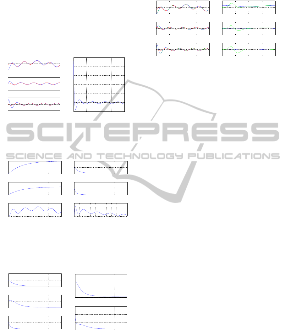
v
1
= v − ˆz
4
, where ˆz
4
is the fourth element of the ex-
tended state vector and is an estimate of disturbance
term z
4
=
˜
d. The associated results are depicted in
Fig. 2 to Fig. 5. It can be observed that the proposed
nonlinear feedback control scheme enables accurate
tracking of the concentration of the P53
∗
protein to
the desirable concentration levels.
0 5 10 15 20
0
20
40
time (h)
P53*
0 5 10 15 20
−50
0
50
time (h)
d/dt P53*
0 5 10 15 20
−50
0
50
time (h)
d
2
/dt
2
P53*
(a)
0 5 10 15 20
0
200
400
600
800
1000
1200
infusion rate
time (h)
u
(b)
Figure 2: Dynamical model with disturbances: (a) nonlin-
ear feedback control of the P53
∗
protein concentration (blue
line) and convergence to the associated setpoints (red lines),
(b) infusion rate as control input.
0 5 10 15 20
10
10.5
time (h)
p53
0 5 10 15 20
0
200
400
time (h)
P53
0 5 10 15 20
0
20
40
time (h)
P53*
(a)
0 5 10 15 20
0
10
20
time (h)
mdm2
0 5 10 15 20
0
10
20
time (h)
MDM2
2 4 6 8 10 12 14 16 18 20
0
100
200
time (h)
N
(b)
Figure 3: Dynamical model with disturbances: (a) variation
of the p53 mRNA concentration, P53 concentration in the
cytoplasm and active P53
∗
concentration, (b) variation of
the mdm2 mRNA concentration, MDM2 concentration in
the cytoplasm and active MDM2
∗
concentration.
0 5 10 15 20
0
10
20
time (h)
e2f1
0 5 10 15 20
0
10
20
time (h)
E2F1
0 5 10 15 20
0
10
20
time (h)
E2F1*
(a)
0 5 10 15 20
0
5
10
15
time (h)
arf
0 5 10 15 20
0
5
10
15
time (h)
ARF
(b)
Figure 4: Dynamical model with disturbances: (a) variation
of the e2f1 mRNA concentration, E2F1 concentration in
the cytoplasm and active E2F1
∗
concentration, (b) variation
of the ar f mRNA concentration, ARF concentration in the
cytoplasm.
0 5 10 15 20
0
20
40
time (h)
P53*
0 5 10 15 20
−50
0
50
time (h)
d/dt P53*
0 5 10 15 20
−50
0
50
time (h)
d
2
/dt
2
P53*
(a)
0 5 10 15 20
−10
0
10
time (h)
d
0 5 10 15 20
−5
0
5
time (h)
d/dt d
0 5 10 15 20
−1
0
1
time (h)
d
2
/dt
2
d
(b)
Figure 5: Dynamical model with disturbances: (a) con-
vergence of the estimates of P53
∗
concentration and of
its derivatives (green lines) to the associated real parame-
ter values (blue lines), (b) estimation of disturbance terms
(green lines) that affect the model and convergence to the
associated real parameter values (blue lines).
6 CONCLUSIONS
A nonlinear feedback control method has been pro-
posed for the p53 protein - mdm2 inhibitor system.
The control scheme is based on differential flatness
theory and the Derivative-free nonlinear Kalman Fil-
ter. The first stage for the design of the control scheme
was the transformation of the initial description of
the system dynamics from a set of complex coupled
nonlinear differential equations into a SISO model of
the canonical Brunovsky form. The transformation
was based on differential flatness theory. The latter
model connected the infusion rate of the chemother-
apy drug (control input) to the concentration of the
P53 protein (system’s output). For the transformed
model the design of state feedback control was possi-
ble. Moreover, to make the control scheme robust to
modeling uncertainty and external disturbances and
to cope with the nonmeasurable elements of the state
vector (derivatives of the P53 protein concentration),
a disturbance estimator was designed with the use of
the Derivative-free nonlinear Kalman Filter. The effi-
ciency of the proposed control scheme was evaluated
through simulation experiments.
REFERENCES
W. Abou-Jaoud´e, M. Chav´es and J. L. Gouz´e, A theoreti-
cal exploration of birhythmicity in the p53-mdm2 net-
work, INRIA Research Report No 7406, Oct. 2010.
M. Bassevile and I. Nikiforov, Detection of abrupt changes:
Theory and Applications, Prentice-Hall, 1993.
S. Bououden, D. Boutat, G. Zheng, J. P. Barbot and F. Kratz,
A triangular canonical form for a class of 0-flat non-
linear systems, International Journal of Control, Tay-
lor and Francis, vol. 84, no. 2, pp. 261-269, 2011.
Controlofthep53Protein-mdm2InhibitorSystemusingNonlinearKalmanFiltering
213

J. Elias, L. Dimitrio, J. Clairambault and R. Natalini, The
p53 protein and its molecular network: modelling
a missing link between DNA damage and cell fate,
Biochimica and Biophysica Acta - Proteins and pro-
teomics, 2013.
M. Fliess and H. Mounier, Tracking control and π-freeness
of infinite dimensional linear systems, In: G. Picci
and D.S. Gilliam Eds.,Dynamical Systems, Control,
Coding and Computer Vision, vol. 258, pp. 41-68,
Birkha¨user, 1999.
M. Jahoor Alam, N. Fatima, G. R. Devi and R. K. Bro-
jen, The enhancement of stability of P53 in MTBP
induced p53-MDM2 regulatory network, Biosystems,
Elsevier, vol. 110, pp. 74-83, 2012.
B. Laroche, P. Martin, and N. Petit, Commande par
platitude: Equations diff´erentielles ordinaires et aux
deriv´ees partielles, Ecole Nationale Sup´erieure des
Techniques Avanc´ees, Paris, 2007.
G. B. Leenders and J. A. Tuszynski, Stochastic and deter-
ministic models cellular p53 regulation, Frontiers of
Oncology, vol. 3, article No 64, 2013.
J. L´evine, On necessary and sufficient conditions for dif-
ferential flatness, Applicable Algebra in Engineering,
Communications and Computing, Springer, vol. 22,
no. 1, pp. 47-90, 2011.
G. Lillacci, M. Boccadoro and P. Valigi, The p53 network
and its control via MDM2 inhibitors: insights from
a dynamical model, Proc. 45th IEEE Conference on
Decision and Control, San Diego, California, USA,
Dec. 2006.
Ph. Martin and P. Rouchon, Syst`emes plats: planifica-
tion et suivi des trajectoires, Journ´ees X-UPS,
´
Ecole
des Mines de Paris, Centre Automatique et Syst`emes,
Mai,1999.
S. K. Peirce and H. W. Findley, Targetting the MDM2-p53
interaction as a therapeutic strategy for the treatment
of cancer, Cell Health and cytoskeleton, Dove Medical
Press, vol. 2, pp. 49-58, 2010.
J. Qi, S. Shao, Y. Shen and X. Gu, Cellular responding
DNA damage: a predictive model of P53 Gene Regu-
latory Networks under continuous ion radiation, Proc.
27th Chinese Control Conference, Kunming Yunnan,
China, July 2008.
J. Wagner, L. Ma, J.J. Rice, W. Hu, A.J. Levine and G.A.
Stolovitzky, p53-mdm2 loop controlled by a balance
of its feedback strength and effective dampening us-
ing ATM and delayed feedback, IEE Proceedings on
Systems Biology, vol. 152, no.3, pp. 109-118, 2005.
G. G. Rigatos and S.G. Tzafestas, Extended Kalman Fil-
tering for Fuzzy Modelling and Multi-Sensor Fusion,
Mathematical and Computer Modelling of Dynami-
cal Systems, Taylor & Francis, vol. 13, pp. 251-266,
2007.
G. Rigatos and Q. Zhang, Fuzzy model validation using the
local statistical approach, Fuzzy Sets and Systems, El-
sevier, vol. 60, no.7, pp. 882-904, 2009.
G. Rigatos, Modelling and control for intelligent industrial
systems: Adaptive algorithms in robotics and indus-
trial engineering, Springer, 2011.
G. Rigatos, Advanced models of neural networks: Nonlin-
ear dynamics and stochasticity in biological neurons,
Springer, 2013.
G. Rigatos and E. Rigatou, A Kalman Filtering approach to
robust synchronization of coupled neural oscillators,
ICNAAM 2013, 11th International Conference of Nu-
merical Analysis and Applied Mathematics, Rhodes,
Greece, Sep, 2013.
P. Rouchon, Flatness-based control of oscillators,
ZAMM Zeitschrift fur Angewandte Mathematik
und Mechanik, vol. 85, no.6, pp. 411-421, 2005
J. Rudolph, Flatness Based Control of Distributed Pa-
rameter Systems, Steuerungs- und Regelungstechnik,
Shaker Verlag, Aachen, 2003.
H. Sira-Ramirez and S. Agrawal, Differentially Flat Sys-
tems, Marcel Dekker, New York, 2004.
BIOINFORMATICS2014-InternationalConferenceonBioinformaticsModels,MethodsandAlgorithms
214
