
A Heuristic Framework for Path Planning the Largest Volume Object
from a Start to Goal Configuration
Evan Shellshear and Robert Bohlin
Fraunhofer Chalmers Centre, Gothenburg, Sweden
Keywords:
Path Planning, Heuristic, Largest Volume.
Abstract:
In this article we present a heuristic algorithm to compute the largest volume of an object in three dimensions
that can move collision-free from a start configuration to a goal configuration through a virtual environment.
The results presented here provide industrial designers with a framework to reduce the number of design
iterations when designing parts to be placed in tight spaces.
1 INTRODUCTION
Being able to determine whether a virtual object can
pass through a virtual environment collision-free is a
fundamental problem in virtual design. Depending on
the exact problem at hand, there exist hundreds of pa-
pers addressing this problem from all sorts of aspects.
In this paper we focus on a lesser studied problem of
utmost importance for industrial designers. We are
interested in being able to compute the largest object
than can travel collision-free from a start configura-
tion to a goal configuration. This academic investi-
gation is motivated by numerous real life problems
and the basic motivation for this article is the virtual
verification and automation of car designs. In partic-
ular, one wants to know if a new car design can pass
through an assembly line without colliding with other
objects and if it does collide, what are the minimal
design changes that need to be made to avoid the col-
lisions. This information can also be used for future
design problems if the environment and trajectory re-
main the same (as is typical for factory installations).
The most important contribution of the results in
this paper is to grant the designer the ability to carry
out product design changes much earlier in the pro-
duction phase. It is well-known that the later the de-
sign changes occur during the production cycle the
more expensive these changes are, (Folkestad and
Johnson, 2002). Hence, the framework presented here
could be used to save significant amounts of money
by allowing designers to figure out correct and allow-
able designs much earlier in the design phase. Typ-
ical applications where computing the non-colliding
design of numerous parts play an important role in-
clude, inter alia, the ability to route and path plan ob-
jects through tight spaces such as engines (Hermans-
son et al., 2012) and other assembly components or
even assembly lines, designing robots for tight spaces
in path planning applications (Spensieri et al., 2013;
Spensieri et al., 2008; Carlson et al., 2013) as well as
almost any other product design scenario where the
assembly of parts occurs. Once the set of colliding
parts has been discovered one can then apply any of
numerous algorithms to effect the necessary design
changes to avoid collisions, (Bj
¨
orkenstam et al., 2012;
Vanderhyde and Szymczak, 2008).
The problem we are interested in can be defined
more exactly as follows. Let a start configuration (po-
sition and orientation) and goal configuration in R
3
be
given. Then we wish find a path from the start config-
uration to the goal configuration that allows an object
of the largest possible volume to pass collision-free
along it. In this paper we will not pursue the ambi-
tious goal of finding the global maximum volume. We
will compute a local maximum volume by adjusting
the positions and orientations of a propitious initial
path. The work presented in this paper extends the
results and algorithms presented in (Shellshear et al.,
2014) and (Ilies and Shapiro, 1999), where the path-
planning object’s path is fixed.
The remainder of this paper is organized as fol-
lows. In the next section we present our algorithm
and its analysis. In the final section we conclude.
264
Shellshear E. and Bohlin R..
A Heuristic Framework for Path Planning the Largest Volume Object from a Start to Goal Configuration.
DOI: 10.5220/0005002102640271
In Proceedings of the 11th International Conference on Informatics in Control, Automation and Robotics (ICINCO-2014), pages 264-271
ISBN: 978-989-758-040-6
Copyright
c
2014 SCITEPRESS (Science and Technology Publications, Lda.)

2 THE ALGORITHM
In this section we present our algorithm to compute a
path that maximizes the volume of an object to pass
collision-free along it. Note that this maximization
is only local and not global. This is because our
method of optimization only considers paths that can
be reached via successive small perturbations of the
clearance maximizing path between the start and goal
configurations. Throughout, unless stated otherwise,
by clearance we mean minimum distance.
The first step of any such algorithm is to define
a start and goal configuration. In addition to the
start and goal configurations, the degrees-of-freedom
(DOF) of the object are important too (LaValle and
Kuffner Jr, 2001). In this paper, we allow the object,
the volume of which is to be maximized, to move with
six DOF, i.e. translations in any direction and any type
of orientation in R
3
.
Given a start and goal configuration, Algorithm
3 computes a volume maximizing path between the
start and goal configuration and returns a voxelized
representation of the volume maximizing object as
well as the path for it to take. We now give an
overview of the main algorithm presented in Algo-
rithm 3 and afterwards we then analyze each of the
most important parts in detail.
The first step of the algorithm is to find a path from
the start configuration to the goal configuration that
will then be locally optimized. Because we want to
maximize the volume of an object to move collision-
free from the start to goal configurations, we choose
initially to find a path that maximizes the volume of
the largest ellipsoid that can pass along it. The choice
of ellipsoid is based on the balance between the many
DOF an ellipsoid has, which can be used to approxi-
mate a given shape, as well as its simplicity.
After having found an initial path that maximizes
the volume of any ellipsoid moving from the start to
goal configuration, we then double the ellipsoid in
each of its three dimensions and voxelize the result.
The larger ellipsoid is then moved along the previ-
ously computed path removing voxels from it as they
collide with the surroundings. We store the set of col-
liding voxels and then working backwards from the
last colliding voxel, we attempt to make local adjust-
ments to prevent each voxel from colliding. This is
presented in pseudocode in the while loop, starting
at line 4 in Algorithm 1, with this new object and
new path. We carry out this while loop until we have
reached some cut-off criterion or maximum number
of iterations. Then we return the best found object
and its path.
After attempting to retain as many colliding vox-
els as possible, we then attempt to add voxels around
the shape computed by Algorithm 1 in Algorithm 2.
This is done by increasing the clearance from each
voxel to its surroundings and adding new voxels next
to voxels that have a large enough clearance.
We now present all three algorithms in detail.
Algorithm 1: AdjustPath(Path, Object, OriginalObject).
1: Input: The current path Path that the current ob-
ject Object is to travel along.
2: Output: A path and object.
3: Let IncreaseVolume be a boolean and set it equal
to true
4: while Iterations < Max Number of Iterations and
IncreaseVolume = true do
5: Move Object along Path and use the last col-
liding cell(s) to adjust the path to prevent the
cell(s) from colliding. Call the adjusted path
AdjustedPath and the object AdjustedObject.
6: if Volume(AdjustedObject) > Volume(Object)
then
7: Ob ject ← Ad justedOb ject.
8: Path ← Ad justedPath.
9: else
10: IncreaseVolume = false
11: end if
12: end while
13: Return Path and Object
Algorithm 2: NewPath(CurrentPath, CurrentObject).
1: Input: The current path CurrentPath that the cur-
rent object CurrentObject is to travel along.
2: Output: A path and object.
3: Path plan CurrentObject from the start to goal
configuration of CurrentPath so as to maximize
the clearance of it to the surroundings and record
the clearance of each boundary voxel. Call this
path Path.
4: V ← Volume(CurrentOb ject).
5: for All boundary voxels of CurrentObject do
6: if Clearance of voxel along whole path > size
of voxel then
7: Add voxels on all free sides of the current
voxel of CurrentObject.
8: end if
9: end for
10: if V < Volume(CurrentOb ject) then
11: CurrentPath ← Path.
12: end if
13: Return CurrentPath and CurrentObject.
AHeuristicFrameworkforPathPlanningtheLargestVolumeObjectfromaStarttoGoalConfiguration
265

Algorithm 3: Computing the volume maximizing path for
a user defined object between the start and goal configura-
tions.
1: Input: A start and a goal configuration as well as
an object that should pass along the path.
2: Output: A voxel representation of the largest ob-
ject that can go from the start to the goal configu-
ration based on the user defined object.
3: Let OptPath be an empty path.
4: Find an initial path from start to goal configura-
tions that maximizes the volume of an ellipsoid.
Set OptPath equal to this path.
5: Voxelize the volume defined by the user and call
it OrigObject. Move OrigObject along the path
from start to goal configurations removing collid-
ing voxels from it. Call the remaining voxelized
object RemObject.
6: Path ← OptPath.
7: Ob ject ← RemOb ject.
8: OptPath, RemOb ject ←
Ad justPath(Path, Ob ject, OrigOb ject)
9: while OptPath 6= Path or RemOb ject 6= Ob ject
do
10: Path ← OptPath
11: Object ← RemObject
12: OptPath, RemOb ject ← NewPath(Path, Ob ject)
13: end while
14: Return OptPath and RemObject.
2.1 Computing the Initial Path
The authors anticipate that a good choice of initial
path for the maximum volume object will play a ma-
jor role in the number of iterations of the while loop in
Algorithm 3 and 1, which both attempt to increase the
volume of the final object. Hence, we have developed
a method of finding a good initial path that comprises
a major part of Algorithm 3 and is the computation in
Step 4 in Algorithm 3.
In finding the initial path we have a number of
choices. One could simply take the clearance maxi-
mizing path, (Geraerts and Overmars, 2005). How-
ever, because one often has significant clearance in
the direction of movement, we chose to find a path
that maximizes the volume of a rotationally symme-
try ellipsoid. Our goal is to produce a path that ex-
ploits additional clearance in at least one dimension,
i.e. the direction of motion. In the following, because
the ellipsoid is rotationally symmetric, we write r for
the radii of the two equal axes (i.e. if we call the radii
r
1
, r
2
and r
3
, then r
2
= r
3
= r). To compute the path
for an ellipsoid with maximal volume, we start with
the path of maximum clearance for a point.
There exist numerous methods to produce a clear-
ance maximizing path between the start and goal con-
figurations. Initially one could use any of numerous
path planning algorithms, (Bohlin and Kavraki, 2000;
LaValle and Kuffner Jr, 2001), to generate an initial
path and then optimize this path to maximize clear-
ance, (Geraerts and Overmars, 2005). Other methods
involve including the clearance maximization criteria
in the path planning algorithm itself, (Zheng et al.,
2011; Kim et al., 2003). However one chooses to
compute the path, we will assume it as given. As
is usual in the path planning literature (Bohlin and
Kavraki, 2000), our path will be defined by a set of
n configurations, {x
i
}, i = 1, .. ., n, with the position
and orientation between configurations x
i
and x
i+1
be-
ing defined by the linear interpolation of the position
and orientation between both configurations.
The reason for us to initially begin with a clear-
ance maximizing path is that it means that the path
will be located on the 3D medial axis, (Geraerts and
Overmars, 2005), between the start and goal configu-
rations. This choice of path as the initial path to lo-
cally optimize is to allow the radii of the ellipsoid,
orthogonal to the direction of motion, to be as large
as possible because they will be constrained by the
minimum distance from the ellipsoid’s path to the sur-
roundings. The reader should note that in real appli-
cations the medial axis can be disconnected and dis-
continuous. Hence, when the ellipsoid travels from
the start to goal configuration, it is only important that
the ellipsoid follows the medial axis along sections of
the path that have low clearance and along other sec-
tions it is less important and the medial axis can be
used more to guide the motion.
Given the initial path that determines the center
point of our ellipsoid, we also wish to determine an
initial orientation of the ellipsoid that maximizes the
volume of the ellipsoid for the current path. With the
assumption on the radii stated earlier (i.e. r
2
= r
3
= r),
we fix the orientation of the first axis of the ellipsoid
to be equal to the tangent of the medial axis. The
tangent has the property that it is ”locally optimal”
because it points in the direction of the next part of
the medial axis path, i.e. to the next point of maximal
clearance, and hence should allow r
1
to be as large as
possible (for the next instantaneous movement).
Given that we now have the center point and orien-
tation of our ellipsoid, all that remains is to compute
the radii that give the maximum volume. To do that
we first create a corridor map of the medial axis as de-
scribed in (Geraerts and Overmars, 2007). We know
that any object contained in this corridor is collision-
free. After having done this we then compute the
maximum value of r
1
, say R, for each configuration
x
i
by finding the first point intersected by a line in the
ICINCO2014-11thInternationalConferenceonInformaticsinControl,AutomationandRobotics
266
direction of the ellipsoid’s first axis’ orientation going
through the center point. One can now use the corri-
dor map to find the maximal values of r for each value
of r
1
, 0 ≤ r
1
≤ R. That is, we continually shorten the
length of the first axis, r
1
, and see how much we can
increase r by shortening r
1
. To make sure that these
values provide a collision-free movement for the el-
lipsoid, we move the ellipsoid along the medial axis
with radii equal to the current r
1
and r. If a colli-
sion occurs, then we reduce r and move the ellipsoid
along the path again continuing in this way until a
value is found for which the combination of r
1
and r
is collision-free. For each value of r
1
, we then save
the maximum, collision-free value of r in a local ta-
ble defining the relationship between r
1
and r at the
configuration x
i
. Once we have completed this com-
putation for all configurations {x
i
}, we then find the
configurations that constrain r
1
and r the most and use
them to choose radii that maximize the volume of el-
lipse given all constraints on r
1
and r. Note that these
choices of radii are not guaranteed to be collision-free
and we take up this point in the coming local opti-
mizations of the ellipsoid’s volume.
The previously computed ellipsoid is restricted in
a number of ways. When finding the largest r
1
possi-
ble we only used the tangent to determine the orien-
tation, which can be less than optimal for paths with
sudden changes in the direction of the path. Hence,
it could be possible that, by slightly deviating from
these orientations and possibly also adjusting the cen-
ter point of our ellipsoid, one can increase the volume
of the ellipsoid. We now introduce a method to in-
crease the volume of the ellipsoid by slightly perturb-
ing its position and orientation so that such a pertur-
bation leads to an increase in volume.
The function we are attempting to increase by lo-
cally perturbing the ellipsoid’s position and orienta-
tion is given in Equation 1. We attempt to maximize
the volume, Equation 1, while making sure that the
ellipsoid is collision-free, Equation 2, and simultane-
ously perturb the ellipsoid’s radii, centerpoint and ori-
entation. This is carried out at each configuration x
i
.
However, when doing this, we first start at the config-
uration x
i
that defines the maximum collision-free val-
ues of r
1
and r and attempt to increase the radii there.
If this succeeds, then we move onto the next configu-
ration that defines the current maximum collision-free
values of r
1
and r. We repeat this until it is no longer
possible to increase r
1
and r.
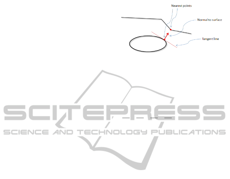
We now explain the notation presented in Equa-
tions 1 and 2. For each configuration x
i
, let p
j
( j =
1, . . . , m), be the points on the ellipsoid that are closest
to the surroundings and let σ
j
stand for the clearance
for each point p
j
. Let the outward surface normals to
Figure 1: Normal to an ellipse’s surface.
the ellipsoid at these points be N
j
, i.e. the vector per-
pendicular to the tangent plane at p
j
and which also
face out of the ellipsoid (see Figure 1). Let c stand for
the ellipsoid’s center point and o stand for the ellip-
soid’s orientation.
maxV (c, o, r
1
, r) (1)
∂p
j
∂c
+
∂p
j
∂o
+
∂p
j
∂r
1
+
∂p
j
∂r
· N
j
≤ σ
j
, j = 1, . . . , m.
(2)
To solve this problem we linearize each of the
functions in Equation 1 and 2. In the following, V
0
is the original volume, A is the first order approxima-
tion to the change in the volume gradient, (p
j
)
0
is the
current p
j
value and P
j
is the first order approxima-
tion to the change in p
j
. We also denote the vector
(dc, do, dr
1
, dr) by dz.
V ≈ V
0
+ Adz (3)
p
j
≈ (p
j
)
0
+ P
j
dz, j = 1, . . . , m. (4)
To these equations we add another equation to
guarantee that between configurations the ellipsoid
will not collide with its surroundings. In the follow-
ing equation let ε
i
stand for the minimum distance
between the ellipsoids and its surrounds between the
current configuration x
i
and the next for the volume
maximizing ellipsoid as computed earlier,
|dc| + r
1
|do| + |dr
1
| + |dr| < ε
i
. (5)
The r
1
that |do| is multiplied by is there to pro-
vide an upper bound on the movement of any point
on the ellipsoid when o changes by do. By letting
V
T
denote the transpose of a vector V , we use these
linearized forms to write the linearized version of the
maximization problem presented in Equation 1 and 2,
with the added collision-free guarantee, as
maxAdz (6)
(N
j
)
T
P
j
dz ≤ σ
j
, j = 1, . . . , m, (7)
|dc| + r
1
|do| + |dr
1
| + |dr| < ε
i
. (8)
The above uses the fact that the slight change in
p
j
, dp
j
= P
j
dz, should fulfill d p
j
· N
j
≤ σ
j
. Another
AHeuristicFrameworkforPathPlanningtheLargestVolumeObjectfromaStarttoGoalConfiguration
267

restriction that we can add that reduces the possible
values of dc is that we only want to look at move-
ments of the ellipse center point, c, that are orthogo-
nal to the path because movements along the path can
be incorporated by applying the maximization prob-
lem there. We define the orthogonal directions to be
orthogonal to the tangent of the medial axis at x, t(x).
Hence our complete optimization problem becomes,
maxAdz (9)
(N
j
)
T
P
j
dz ≤ σ
j
, j = 1, . . . , m, (10)
dc ·t(c) = 0, (11)
|dc| + r
1
|do| + |dr
1
| + |dr| < ε
i
. (12)
In the previous set of equations, Equation 10 guar-
antees that, as we optimize the ellipsoid’s shape at the
current configuration, the ellipsoid will adjust it’s po-
sition in a locally optimal way. Equation 12 guaran-
tees that these changes are so that the optimized el-
lipsoid has a shape that is guaranteed to be collision-
free between the current configuration and the next
(by definition of ε
i
).
To compute A and P
j
we proceed as follows. As is
clear changing the position or orientation of the ellip-
soid does not effect the volume. However increasing
r
1
and r does. As the volume of the ellipsoid is equal
to:
4
3
πr
1
r
2
, (13)
the reader can check that the linearization of A is then
equal to (dz is 9 element vector: 3 elements for small
position changes, 3 elements for the small orientation
changes, 1 for each radii change)
(0, 0, 0, 0, 0, 0,
4
3
πr
2
,
4
3
πr
1
r,
4
3
πr
1
r). (14)
The P
j
are computed by noticing that movements in
the position of the ellipsoid directly affect the corre-
sponding position of the points p
j
, hence we just add
their contributions to the points. When a point is ro-
tated through Euler angles α, β and γ ≈ 0, then we
can use the following linearization of the rotation for
small angles to compute the movement of the point
(N
¨
uchter et al., 2010),
1 −γ β
γ 1 −α
−β α 1
. (15)
Computing the effects of increases or decreases in the
radii on the coordinates of p
j
can be carried out as
follows: assume first of all that the ellipsoid axes are
aligned with the Cartesian axes and that the ellipsoid
is located at the origin (although the location of the
ellipsoid does not effect the size of the increase or de-
crease in any of the radii). To simplify the coming
notation we consider the case where we only adjust
r
1
, the other cases being analogous. Note that one
can use the parametrization of a point on an ellipsoid
to compute its movement in the direction of an axis
caused by changes in the radii. Points on an ellipsoid
can be represented by the following parametric equa-
tions,
x = r
1
cosu cos v (16)
y = r cos u sin v (17)
z = r sin u, (18)
where −
π
2
≤ u ≤
π
2
and −π ≤ v ≤ π. Hence for a
point at (x, y, z) with angles (u, v) = (θ, φ) an increase
in radius of ∆r
1
results in a movement of the r
1
axis
of ∆r
1
cosθsin φ.
Hence, given the orientation (in Euler angles) of
the ellipsoid as (α,β, γ) (with corresponding rotation
matrices R(α), R(β) and R(γ)), the final movement of
the point, located at (θ, φ) in parametric coordinates,
caused by the adjustment in the first radius is equal to
∆r
1
∆
1
, whereby
∆
1
:= R(α)R(β)R(γ)(cosθsin φ, 0, 0). (19)
Similarly for the other two radii, let ∆
k
with k = 2, 3
be the adjustment for the radius corresponding to the
second and third ellipsoid axis respectively. The cor-
rectness of this is guaranteed by the fact that for a
rotation R, vector v and scalar λ, R(λv) = λRv. Hence
P
j
has the form
1 0 0 1 −γ β ±(∆
1
)
x
±(∆
2
)
x
±(∆
3
)
x
0 1 0 γ 1 −α ±(∆
1
)
y
±(∆
2
)
y
±(∆
3
)
y
0 0 1 −β α 1 ±(∆
1
)
z
±(∆
2
)
z
±(∆
3
)
z
where the plus or minus is determined by where p
j
is
located with respect to the corresponding axis plane
and (∆
k
)
x
stands for the x coordinate of the ∆
k
vector
(similarly for y and z).
If the previous optimization is successful, then we
can repeat it until no more increases in the ellipsoid’s
volume are possible. Figure 2 demonstrates the pre-
vious optimization applied to an ellipse.
2.2 Voxelizing the Ellipsoid
In this section we explain Step 5 in Algorithm 3. To
make sure that we are able to gain the maximum bene-
fit from the algorithms we double the ellipsoid’s radii
in all three dimensions and then voxelize the resulting
ellipsoid. We voxelize the entire volume with vox-
els of a fixed size, say δ > 0. The choice of delta
is influenced by the available computational power.
A smaller δ results in more tests and hence a higher
computational demand. To voxelize the ellipsoid, we
find the bounding box of the ellipsoid and divide the
ICINCO2014-11thInternationalConferenceonInformaticsinControl,AutomationandRobotics
268
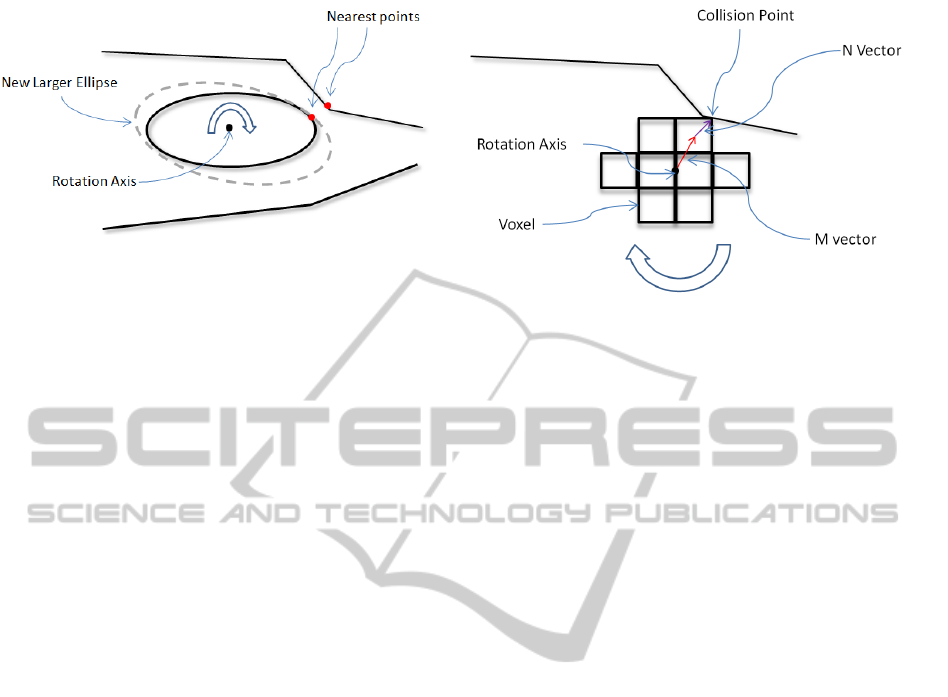
Figure 2: Increasing the ellipse’s volume while rotating and
translating it.
box into small voxels and find supercover of the ellip-
soid (i.e. all voxels that meet the ellipsoid, (Cohen-Or
and Kaufman, 1995)) . These voxels will then de-
fine a (26,6)-neighbor closed surface (Cohen-Or and
Kaufman, 1995) (i.e. any of the 26 voxels surround-
ing a voxel are a neighbor to the voxel if they are
non-empty and all empty voxels surrounding a voxel
are neighbors if they are adjacent to any one of the
voxel’s faces) because they voxelize the closed sur-
face defined by the ellipsoid. We then remove all vox-
els of the bounding box that are not part of the bound-
ary or inside of the object. We do this by finding all
boundary voxels of the voxelized bounding box of the
ellipsoid that are not intersected by the ellipsoid. We
then carry out a breadth-first search of all such voxel’s
26-neighbors that are not part of the supercover of the
voxels intersected by the ellipsoid.
2.3 Path Planning with the Voxelized
Ellipsoid on the New Path
After having computed the initial path and voxeliza-
tion of the ellipsoid, we then move our voxelized ob-
ject along the initial path (given by OptPath in Algo-
rithm 3) adjusting its configuration to remove colli-
sions. This is the content of Algorithm 1.
To move the voxelized ellipsoid along the path and
find any voxel colliding with surroundings, we use the
technique in (Shellshear et al., 2014) (although one
could also use the algorithms presented in (Ilies and
Shapiro, 1999)). The method presented in (Shellshear
et al., 2014) computes the set of all colliding voxels
along the path from the start to goal configurations.
The technique presented in (Shellshear et al., 2014) is
also able to find the colliding voxels, which we will
require below. For simplicity, in the following sec-
tions we will call the remaining voxelized volume the
voxelized ellipsoid even though the remaining shape
after removing all colliding voxels may not look like
an ellipsoid at all.
As the voxelized ellipsoid moves along the path
Figure 3: Rotating the voxelized ellipsoid (in 2D) to prevent
collisions with voxels.
we find all colliding voxels and store them. Once
the voxelized ellipsoid has completed the motion, we
then use the set of colliding voxels to locally adjust
the path to try and avoid collision along the path. We
start with the last colliding voxel along the path. We
know that if we can locally adjust (these adjustments
are described in more detail below) the movements
of the voxelized ellipsoid during this part of the path
so that the voxel is not colliding and does not intro-
duce any new collisions, then the voxel will not col-
lide with anything else on the path before this point
because it was not colliding previously. Hence each
local adjustment can be done without affecting previ-
ous collisions along the path. So if we are success-
fully able to locally adjust the path, then we let the
new set of voxels travel along the path from the cur-
rent configuration until the end and see if the newly
added voxel collides with anything else. If it does
collide with something, then we repeat the previous
local adjustments to the path at the point of collision
and repeat the aforementioned.
We now describe how to carry out these local ad-
justments. To locally adjust the set of voxels, we cre-
ated a number of slight adaptations on a methods typ-
ically used in computer graphics to remove penetra-
tions, (Zachmann et al., 2000). So to locally adjust
the set of voxels so that they are no longer collid-
ing, we developed four different strategies. The first
is the simplest and involves attempting to rotate the
voxelized ellipsoid to remove the collision. Let N be
the vector pointing from the centerpoint of the collid-
ing voxel to the point of contact with the surround-
ings and M be the vector from the voxelized ellip-
soid’s centerpoint to the colliding voxel’s centerpoint,
see Figure 3. We then rotate the voxelized ellipsoid
away from the colliding voxel around the axis equal
to the cross product of N and M and passing through
the objects centerpoint. We do this until another col-
lision occurs or the voxel is no longer colliding. If
AHeuristicFrameworkforPathPlanningtheLargestVolumeObjectfromaStarttoGoalConfiguration
269

rotating in such a way cannot move the voxelized el-
lipsoid into a collision-free configuration, then we try
translating the voxelized ellipsoid in the direction of
the colliding voxel’s centerpoint to the voxelized el-
lipsoid’s centerpoint until the same happens. If nei-
ther works then we attempt to translate (in the same
direction as before) until a new collision happens and
then try to rotate as before and vice versa.
We then carry this out working through the col-
liding voxels always looking at the one that collided
previously (i.e. collided before the current one we are
analyzing). We do this until some cut-off criterion
is reached or until the previous attempt to prevent the
voxel from colliding failed at which point we stop try-
ing to add voxels.
2.4 Path Plan with the Voxelized
Ellipsoid and Adding Voxels
Around Boundary Voxels
We now explain the content of Algorithm 2. In this
algorithm we path plan with the voxelized ellipsoid,
computed from Algorithm 1. We plan a path so that
the path maximizes the clearance from the voxelized
ellipsoid to its surroundings. Once we have found the
clearance maximizing path for our voxelized ellipsoid
with any suitable algorithm, (Zheng et al., 2011; Kim
et al., 2003), we then also measure the minimum dis-
tance from each boundary voxel to the surroundings
along the path. This can be efficiently achieved via
any number of methods, e.g. bounding volume hierar-
chies (Larsen et al., 1999), distance fields (Zachmann
et al., 2000), etc. For each boundary voxel we save
the minimum distance found over the entire path.
After completing this (Step 3 in Algorithm 2), we
then have a list of minimum distances for all voxels
in the set of boundary voxels. We wish to now add
voxels to all sides of a given boundary voxel (that are
not already occupied by boundary voxels), that has
a large enough clearance to guarantee that the newly
added voxels will not collide with the surroundings
on the current path. To provide this guarantee we
only add voxels to all unoccupied 6-neighbor sides
of a voxel if the clearance of the voxel to the sur-
roundings is greater than or equal to the side length
but less than a face diagonal of the voxel. If the clear-
ance is greater than or equal to a face diagonal of the
voxel but less than the major diagonal of the voxel,
then we add all unoccupied 18-neighbors, (Cohen-Or
and Kaufman, 1995), around the voxel. Otherwise if
the clearance is greater than or equal to the major di-
agonal of the voxel then we add voxels to all unoccu-
pied 26-neighbors, (Cohen-Or and Kaufman, 1995),
of the current voxel. By adding voxels in this fash-
ion we can guarantee that the newly added voxels are
collision-free. This is because the minimum distance
from any part of the newly added voxel will be less
than the current voxel’s clearance.
After carrying out this part of the algorithm, the
final computed object is a set of voxels approximating
the largest object that can pass collision-free from the
start to goal configurations.
3 PRACTICAL
IMPLEMENTATION DETAILS
Due to space limitations we present a possible prac-
tical implementation of the previous results but not
actual simulation results. Such results will be pre-
sented in a future publication. In each step requiring
path planning the maximimum clearance, the algo-
rithm in (Kim et al., 2003) can be used. To compute
the pertubations of the initial ellipsoid to maximize
its volume, a suitable optimization method would be
to solve it via linear programming using tools such
as (COIN-OR, 2014). Voxelizing the ellipsoid can be
carried out using the straight-forward implementation
from (Cohen-Or and Kaufman, 1995). To compute
the maximum volume along the new path given the
voxelization, the fast algorithm presented in (Shell-
shear et al., 2014) can be used. Finally to quickly
compute distances, the efficient PQP package can be
used, (Larsen et al., 1999). While each of these previ-
ous algorithms has been demonstrated to be fast, the
running time of the algorithm is expected to be deter-
mined mostly by the iterations in Algorithm 1.
4 CONCLUSIONS
In this article we have presented a heuristic to solve
the designer’s problem of determining the maximum
volume object that can be path planned from a given
start configuration to a goal configuration. The paper
fills an important gap at the intersection of many ar-
eas of research as outlined in the introduction. In ad-
dition, while developing the algorithms, the authors
paid attention to using well-known algorithms and
data structures that have been demonstrated to be ef-
ficient in practice. Hence, we would expect that an
implementation of the algorithms and ideas presented
here should not produce computationally intractable
problems.
In future work we intend to implement the algo-
rithms presented here as well as address practical is-
sues that arise during their implementation. Future
ICINCO2014-11thInternationalConferenceonInformaticsinControl,AutomationandRobotics
270

work will also address trying to find the globally vol-
ume maximizing path among all paths from the start
to the goal configuration. In addition, we took only
strictly better improvements to the volume of the ob-
ject in Step 10 in Algorithm 2 and Step 6 in Algorithm
1. A further avenue for investigation could be to re-
place this with a simulated annealing style optimiza-
tion to allow non-optimal adjustments so that one has
the possibility of escaping local maxima.
ACKNOWLEDGEMENTS
This work was carried out at the Wingquist Labora-
tory VINN Excellence Centre, and is part of the Sus-
tainable Production Initiative and the Production Area
of Advance at Chalmers University of Technology. It
was supported by the Swedish Governmental Agency
for Innovation Systems.
REFERENCES
Bj
¨
orkenstam, S., Segeborn, J., Carlson, J. S., and Bohlin, R.
(2012). Assembly verification and geometry design
by distance field based shrinking. In 4th CIRP Con-
ference on Assembly Technology and Systems-CATS
2012, University of Michigan, Ann Arbor, USA on
May 21-23, 2012.
Bohlin, R. and Kavraki, L. (2000). Path planning using lazy
prm. In IEEE International Conference on Robotics
and Automation, volume 1, pages 521–528. IEEE.
Carlson, J. S., Spensieri, D., S
¨
oderberg, R., Bohlin, R., and
Lindkvist, L. (2013). Non-nominal path planning for
robust robotic assembly. Journal of manufacturing
systems, 32(3):429–435.
Cohen-Or, D. and Kaufman, A. (1995). Fundamentals of
surface voxelization. Graphical models and image
processing, 57(6):453–461.
COIN-OR (2014). COmputational INfrastructure for Oper-
ations Research. http://www.coin-or.org/.
Folkestad, J. E. and Johnson, R. L. (2002). Integrated rapid
prototyping and rapid tooling (irprt). Integrated Man-
ufacturing Systems, 13(2):97–103.
Geraerts, R. and Overmars, M. H. (2005). On improv-
ing the clearance for robots in high-dimensional con-
figuration spaces. In Intelligent Robots and Sys-
tems, 2005.(IROS 2005). 2005 IEEE/RSJ Interna-
tional Conference on, pages 679–684. IEEE.
Geraerts, R. and Overmars, M. H. (2007). The corridor
map method: Real-time high-quality path planning.
In Robotics and Automation, 2007 IEEE International
Conference on, pages 1023–1028. IEEE.
Hermansson, T., Bohlin, R., Carlson, J. S., and S
¨
oderberg,
R. (2012). Automatic path planning for wiring harness
installations (wt). In 4th CIRP Conference on Assem-
bly Technology and Systems-CATS 2012, University of
Michigan, Ann Arbor, USA on May 21-23, 2012.
Ilies, H. T. and Shapiro, V. (1999). The dual of sweep.
Computer-Aided Design, 31(3):185–201.
Kim, J., Pearce, R. A., and Amato, N. M. (2003). Ex-
tracting optimal paths from roadmaps for motion plan-
ning. In Robotics and Automation, 2003. Proceed-
ings. ICRA’03. IEEE International Conference on,
volume 2, pages 2424–2429. IEEE.
Larsen, E., Gottschalk, S., Lin, M. C., and Manocha, D.
(1999). Fast proximity queries with swept sphere vol-
umes. Technical report, Technical Report TR99-018,
Department of Computer Science, University of North
Carolina.
LaValle, S. and Kuffner Jr, J. (2001). Randomized kin-
odynamic planning. The International Journal of
Robotics Research, 20(5):378–400.
N
¨
uchter, A., Elseberg, J., Schneider, P., and Paulus, D.
(2010). Linearization of rotations for globally con-
sistent n-scan matching. In IEEE International Con-
ference on Robotics and Automation (ICRA), page 7.
Shellshear, E., Tafuri, S., and Carlson, J. (2014). A multi-
threaded algorithm for computing the largest non-
colliding moving geometry. Computer-Aided Design,
49(0):1 – 7.
Spensieri, D., Bohlin, R., and Carlson, J. S. (2013). Coordi-
nation of robot paths for cycle time minimization. In
CASE, pages 522–527.
Spensieri, D., Carlson, J. S., Bohlin, R., and S
¨
oderberg, R.
(2008). Integrating assembly design, sequence opti-
mization, and advanced path planning. ASME Confer-
ence Proceedings, (43253):73–81.
Vanderhyde, J. and Szymczak, A. (2008). Topological sim-
plification of isosurfaces in volumetric data using oc-
trees. Graphical Models, 70(1):16–31.
Zachmann, G. et al. (2000). Virtual Reality in Assem-
bly Simulation: Collision Detection, Simulation Algo-
rithms, and Interaction Techniques. Fraunhofer-IRB-
Verlag.
Zheng, L., Cho, Y.-K., Liu, X., and Wang, W. (2011). Cvt-
based 2d motion planning with maximal clearance. In
Robotics and Automation (ICRA), 2011 IEEE Interna-
tional Conference on, pages 2281–2287. IEEE.
AHeuristicFrameworkforPathPlanningtheLargestVolumeObjectfromaStarttoGoalConfiguration
271
