
Complete Stiffness Model for a Serial Robot
Alexandr Klimchik
1,2
, Stephane Caro
2,3
, Benôit Furet
2,4
and Anatol Pashkevich
1,2
1
Ecole des Mines de Nantes, 4 rue Alfred-Kastler, 44307 Nantes, France
2
Institut de Recherches en Communications et Cybernétique de Nantes, UMR CNRS 6597, Nantes, France
3
Centre National de la Recherche Scientifique (CNRS), Paris, France
4
Université de Nantes, quai de Tourville, 44035 Nantes, France
Keywords: Robot Calibration, Elastostatic Identification, Stiffness Modeling, Parameter Identifiability.
Abstract: The paper addresses a problem of robotic manipulator calibration. The main contributions are in the area of
the elastostatic parameters identification. In contrast to other works, the considered approach takes into ac-
count elastic properties of both links and joint. Particular attention is paid to generation of the complete and
irreducible stiffness model that is suitable for the identification. To solve the problem, physical and algebra-
ic model reduction methods are proposed. They are based on taking into account the physical properties of
the manipulator elements and structure of the corresponding observation matrix. The advantages of the de-
veloped approach are illustrated by an application example that deals with elastostatic calibration of an in-
dustrial robot.
1 INTRODUCTION
Industrial robots are gradually finding their niche in
manufacturing, replacing less universal and more
expensive CNC-machines. Application area of ro-
bots is constantly growing, they begin to be used not
only for the assembly and pick-and-place operations,
but also for the machining. The latter requires spe-
cial attention to the accuracy of the model, which is
used to control the manipulator movements. Fur-
thermore, for this process, the robot is usually sub-
ject to essential external loading caused by the ma-
chining force that may lead to non-negligible deflec-
tions of the end-effector (Dépincé and Hascoët,
2006) and, accordingly, degrade the quality of the
final product. This issue becomes extremely im-
portant in the aerospace industry, where the accura-
cy requirements are very high. In this case, the ma-
nipulator stiffness modeling and corresponding error
compensation technique are the key points (Karan
and Vukobratović, 1994; Kövecses and Angeles,
2007), where in addition to accurate geometric mod-
el a sophisticated elastostatic one is required.
In practice, the robot positioning accuracy can be
improved by means of either on-line or off-line error
compensation techniques (Abele, Schützer et al.,
2012; Chen, Gao et al., 2013). Usually geometric
errors (such as offsets and link lengths) can be effi-
ciently compensated by modifying internal parame-
ters of the robot controller (Mooring, Roth et al.,
1991). In contrast, the compliance errors have to be
compensated via modification of the controller in-
puts. In such a case, an off-line error compensation
technique is aimed at adjusting the target trajectory
in accordance with the errors to be compensated and
the geometric model used in the robot controller
(Klimchik, Pashkevich et al., 2013). It is evident that
the efficiency of the latter approach is quite sensitive
to the model completeness and the accuracy of its
parameters.
To achieve desired degree of accuracy, the ma-
nipulator model should be calibrated for each partic-
ular manipulator (Meggiolaro, Dubowsky et al.,
2005). In modern robotics, there exist a number of
techniques that allow user to identify geometric and
elastostatic parameters of either serial or parallel
manipulators. In general, classical calibration proce-
dure contains four basic steps: modeling, measure-
ment, identification and implementation (Roth,
Mooring et al., 1987). The first step is aimed at de-
velopment of a model, which is accurate enough and
also is suitable for the identification (i.e. without re-
dundant parameters that can cause the convergence
breakdown). At the following step, the measure-
ments data are obtained. These data can be gotten
192
Klimchik A., Caro S., Furet B. and Pashkevich A..
Complete Stiffness Model for a Serial Robot.
DOI: 10.5220/0005098701920202
In Proceedings of the 11th International Conference on Informatics in Control, Automation and Robotics (ICINCO-2014), pages 192-202
ISBN: 978-989-758-040-6
Copyright
c
2014 SCITEPRESS (Science and Technology Publications, Lda.)
using open-loop and closed-loop methods (Takeda,
Shen et al., 2004; Nubiola and Bonev, 2013). The
identification step is aimed at tuning the model pa-
rameters in accordance with the experimental data.
The last step, implementation, deals with modifica-
tion the robot control software in accordance with
the identified parameters.
In the manipulator stiffness modeling, there are
currently three main approaches: the Finite Element
Analysis (FEA), the Matrix Structural Analysis
(MSA), and the Virtual Joint Method (VJM). As fol-
lows from our experience, the VJM method (Alici
and Shirinzadeh, 2005; Klimchik, Chablat et al.,
2014) provides reasonable trade-off between the
model accuracy and computational complexity and
will be further used in this paper. It is based on the
extension of the traditional rigid model by adding
the virtual joints describing the elastic deformations
of the links, joints and actuators.
It should be mentioned that calibration of the
elasto-static model is much more difficult compared
to the geometric one. For a simple case, when only
elasticity of the actuated joints is taken into account,
an efficient approach has been proposed in (Dumas,
Caro et al., 2011), but this simplification does not
allow describing some important deflections of the
end-effector. More sophisticated model describing
both the joint and link elasticity can be developed
use CAD-based technique proposed in our previous
work (Klimchik, Pashkevich et al., 2013). However,
this model includes huge number of parameters that
cannot be identified separately using conventional
measurement data describing the end-effector de-
flections caused by external force/torque. It means
that from mathematical point of view, this technique
may produce redundant models that are not suitable
for calibration.
Similar problem is also known in geometric cali-
bration where the concept of complete-irreducible-
continues model has been introduced (Khalil and
Dombre, 2004). However, in elastostatic calibration
there is an additional difficulty caused by huge
number of model parameters (258 for 6 dof manipu-
lator) and essential difference in their magnitudes.
For this reason, this paper deals with developing
stiffness model suitable for identification and pro-
poses model reduction methods that allow obtaining
reliable results in industrial environment.
It is worth mentioning that the adopted approach
deals with quasi-static modeling that is motivated by
the considered application area. In particular, it is
assumed that trajectory tracking compensation does
not takes into account dynamic effects and load dis-
turbances over frequencies.
To address the above mentioned problem, the
remainder of the paper is organized as follows. Sec-
tion 2 presents the stiffness modeling background
and problem statement. In Section 3, the developed
model reduction methods are presented. Section 4
contains application examples that illustrate ad-
vantages of the proposed technique. And finally,
Section 5 summarizes the main contributions of the
paper.
2 THEORETICAL
BACKGROUND AND
PROBLEM STATEMENT
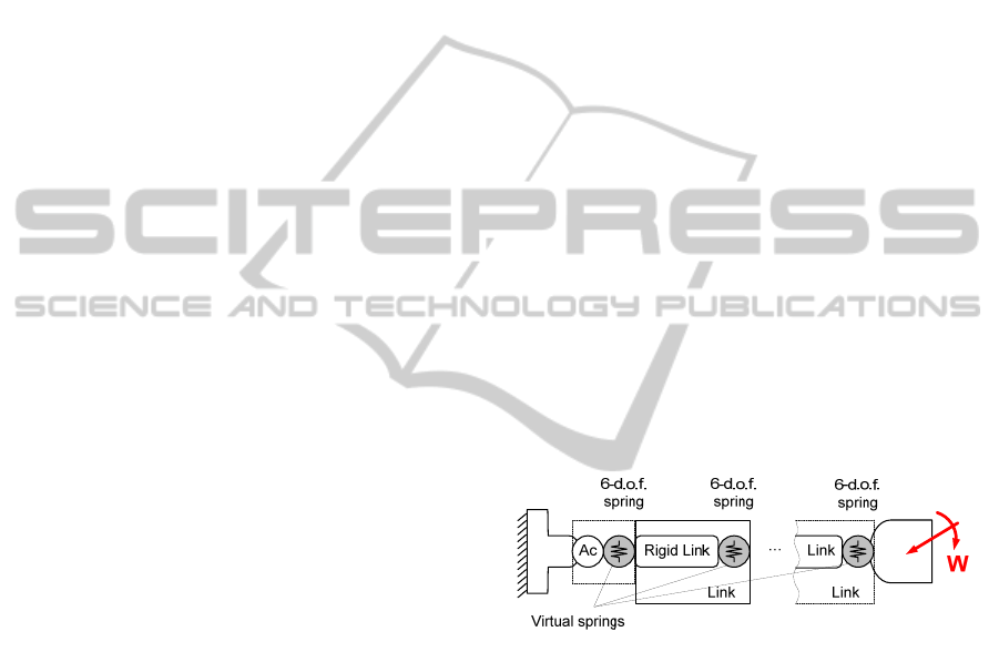
Let us consider an elastostatic model of a general
serial manipulator, which consists of a fixed “Base”,
a serial chain of flexible “Links”, a number of flexi-
ble actuated joints “Ac” and an “End-effector” (0).
In order to describe the stiffness of the considered
manipulator, let us apply the virtual joint method
(VJM), which is based on the lump modeling ap-
proach. According to this approach, the rigid model
should be extended by adding localized spring de-
scribing links elasticity. Besides, in order to take in-
to account the stiffness of the control loop, the virtu-
al springs should be included in the actuated joints.
Figure 1: VJM model of serial robot.
For the considered manipulator the force-
deflection relation for given robot configuration
q
is defined by the Cartesian stiffness matrix
C
K as
C
·Δ
WK t
(1)
In these equations, the end-effector displacement
Δt
is treated as the model input and the external wrench
W
is the model output. The stiffness matrix
C
K
can be computed as follows
1
1T
C θθθ
KJKJ
(2)
Here, the Jacobian matrix
θ
J depends on the manip-
ulator configuration
q
and can be computed as a
partial derivative of the end-effector location with
CompleteStiffnessModelforaSerialRobot
193

respect to a set of desired virtual joint coordinates
θ . Expression (2) allows us to compute the Carte-
sian stiffness matrix assuming that the matrix
(1) (2)
θθθ
( , , ...)diagKKK
, defining elastostatic
properties of the manipulator links/joins is given.
However, in practice, the matrices
(i)
θ
,1,2,...i K
are unknown and should be identified from relevant
experiments.
To estimate the desired matrices describing elas-
ticity of the manipulator components (i.e., compli-
ances of the virtual springs), the elastostatic model
(1) should be rewritten as
(i) (i) (i)T
θθθ
1
·
n
i
JkJtW
(3)
where the matrices
(i) (i) 1
θθ
()
kK
denote the
link/joint compliances that should be identified via
calibration, and the matrices
(i)
θ
J
are corresponding
sub-Jacobians obtained by the fractioning of the ag-
gregated Jacobian
(1) (2)
θθθ
[,,...]
TT
T
JJJ .
In the case when the matrices
(i)
θ
k
are known
the end-effector deflections Δt caused by external
loading W can be compensated by means of either
on-line or off-line error compensation techniques
(Lo and Hsiao, 1998; Klimchik, Bondarenko et al.,
2014). Usually main geometric errors (such as off-
sets and link lengths) can be efficiently compensated
by modifying internal parameters of the robot con-
troller (Mooring, Roth et al., 1991). In contrast, the
compliance errors have to be compensated via modi-
fication of the controller inputs. Relevant on-line
compensation strategy requires external measure-
ment system that continuously provides the end-
effector coordinates, which are compared with the
computed ones and the differences are used for ad-
justing the input trajectory (Lu and Lin, 1997).
However, suitable measurement systems are quite
expensive and often cannot ensure tracking the ref-
erence point in a whole robot workspace. Moreover,
behavior of some technological processes hampers
the end-effector observability (cutting chip in mill-
ing, for instance) and may damage the measurement
equipment. In such a case, an off-line error compen-
sation technique looks more reasonable; it is aimed
at adjusting the target trajectory in accordance with
the errors to be compensated and the geometric
model used in the robot controller (Chen, Gao et al.,
2013; Klimchik, Pashkevich et al., 2013).
However for the majorit of industrial robots the
values of compliance matrices
(i)
θ
k
should be identi-
fied from the dedicated experimental study. So, for
the identification purposes, this expression should be
transformed into more convenient form, where all
desired parameters (elements of the matrices
(i)
θ
, 1, 2,...i k
) are collected in a single vector
(1) (1) ( )
θ11 θ12 θ66
(, ,...)
n
kk kπ
. It yields the following linear
equation
·
tAπ
(4)
where
1212
[ , ,...., ]
TT
m
T
m
AJJWJJWJJW
(5)
is so-called observation matrix that defines the map-
ping between the unknown compliances
π and the
end-effector displacements
t under the loading
W for the manipulator configuration
q . In the ob-
servation matrix
A the subscript defines the pa-
rameters set for which the observation matrix is
computed. Here, the vectors
i
J are the columns of
the matrix
θ
J , i.e.
θ 12
[ , ,...., ]
m
JJJ J.
Taking into account that the calibration experi-
ments are carried out for several manipulator con-
figurations defined by the actuated joint coordinates
,1,
j
jmq
, the system of basic equations for the
identification can be presented in the following form
;1·,
jjj
jm
πεAt
(6)
where
j
ε
describes the measurement noise impact.
Further, using these notations and assigning proper
weights for each equation, the identification can be
reduced to the following optimization problem
1
()()mi
n
m
TT
jj jj
j
F
π
A π tAη tηπ
(7)
where
η
is the matrix of weighting coefficients that
normalizes the measurement data. In practice, the
matrix
η
is used for two main purposes: (i) to avoid
the problem of non-homogeneity due to different
units of equations in the system (6) (position and
orientation components, in this particular case) and
(ii) to give higher weights for the measurements
whose precision is obviously higher. An example of
such an approach has been given in (Klimchik, Wu
et al., 2013). Relevant minimization (7) yields the
following solution
1
11
ˆ
·
mm
TT TT
j
jjj
jj
π AA A tηη ηη
(8)
If the measurement noise is Gaussian (as it is as-
sumed in conventional calibration techniques), ex-
pression (8) provides us with an unbiased estimates
ICINCO2014-11thInternationalConferenceonInformaticsinControl,AutomationandRobotics
194

for which
ˆ
E ππ.
It is clear that expression (8) gives reliable esti-
mates of the parameters π if and only if the matrix
1
1
m
TT
j
j
j
A ΣΣA
is invertible. It leads to the
problem of the parameter identifiability that have
been studied by a number of authors for the problem
of geometrical calibration (Pashkevich, 2001; Khalil
and Dombre, 2004). Relevant techniques are based
on the information matrix rank analysis. However,
they cannot be directly applied for the case of elasto-
static calibration.
Let us assume that the vector of desired elasto-
static parameters
π should be identified from the set
of the linear equations (4) whose least square solu-
tion is defined by the expression (8). Depending on
the matrix set
j
A , corresponding system of line-
ar equations can be solved for
π
either uniquely or
may have infinite number of solutions. In general, if
the information matrix is rank-deficient, a general
solution of the system (6) can be presented in the
following form
ˆ
··
π AIBAAλ
(9)
where the superscript "+" denotes the Moore–
Penrose pseudo-inverse,
1
m
TT
j
j
j
ηηAAA
,
1
m
TT
j
j
j
ηηBAt
and λ is an arbitrary vector
of the same size as
π
. So, all desired parameters
contained in the vector
π
can be divided into three
non-overlapping groups (Pashkevich, 2001):
G1: Identifiable parameters that can be obtained
from (9) in unique way;
G2: Non-identifiable parameters that cannot be
computed uniquely from (9) and do not influence on
the right-hand side of the equation (4);
G3: Semi-identifiable parameters that are also
cannot be computed uniquely but have influence on
the right-hand side of the equation (4).
To present typical examples of the parameters
belonging to the groups G1, G2 and G3, it is possi-
ble to use the ideas similar to geometrical calibra-
tion. For instance, the elastostatic parameters of the
actuated joints and adjacent links are redundant in
their totality and belong to the group G3. Besides, if
the loading direction cannot be altered, a number of
parameters belong to the group G2 and cannot be
identified from the corresponding experimental data.
So, complete and irreducible model should contain
all parameters from the group G1 and partially pa-
rameters of the group G3.
Hence, to obtain reliable stiffness model that is
suitable for calibration, it is necessary to develop
dedicated model reduction techniques and relevant
rules allowing us to minimize the number of pa-
rameters to be estimated and to reconstruct the orig-
inal VJM-based model from these data taking into
account mathematical relations between the model
parameters caused by their physical sense.
3 MODEL REDUCTION
3.1 Physical Approach
Straightforward stiffness modeling approach pro-
vides the exhaustive but redundant number of pa-
rameters to be identified. For instance, each links is
described by a 6 6
matrix that includes 36 parame-
ters that are treated as independent ones. However,
as follows from physics, number of pure physical
parameters is essentially lower. Hence, there are
strong relations between these 36 parameters but this
fact is usually ignored in elastostatic calibration. Be-
sides, due to fundamental properties of conservative
system, the desired compliance matrices should be
strictly symmetrical and positive-definite. In addi-
tion, for typical manipulator links, the compliance
matrices are sparsed due to the shape symmetry with
respect to some axis, but this property is not taken
into account also in the identification of the elasto-
static parameters.
To use the advantages of the compliance matrix
properties and to increase the identification accura-
cy, three simple methods can be applied that allow
us to reduce the number of parameters to be comput-
ed in the identification procedure (8). They can be
treated as the physics-based model reduction tech-
niques and formalised in the following way.
M1:Symmetrisation. For all compliance matri-
ces
k to be identified, replace the pairs of symmet-
rical parameters
,
ij ji
kk
by a single one
,
ij
ki j
.
For each link, this reduction procedure is equiva-
lent to re-definition of the model parameters vector
in the following way
·
π M π
(10)
where the binary matrix
M of size 36 21 de-
scribes the mapping from the original to reduced pa-
rameter space. It can be proved that corresponding
basic expression for the identification (4) can be re-
written as
·
π
At π
(11)
CompleteStiffnessModelforaSerialRobot
195

where ·
ππ
AAM denotes the reduced observation
matrix. The later can be also computed as
θ 1 θθ2 θθ21 θ
[],,...
TT T
π
AJω JwJω Jw Jω Jw
(12)
where
12
, ,...ωω
denote the binary matrices of size
66 for which non-zero elements (i.e. equal to 1)
are located in the following way: for the parameter
l
corresponding to the matrix elements
,
ij
ki j
,
the non-zero elements are
1
ij ji
. It is clear
that this idea allows us to reduce the number of links
compliance parameters from 36 to 21 (and from 258
to 153 for the entire 6 d.o.f. manipulator).
M2:Sparcing. For all compliance matrices k to
be identified, eliminate from the set of unknowns the
parameters
ij
k
corresponding to zeros in the stiff-
ness matrix template
0
k
derived analytically for the
manipulator link with similar shape.
To obtain a desired template matrix, is conven-
ient to use any realistic link-shape approximation.
For example using the trivial beam (Timoshenko and
Goodier, 1970), the desired template can be present-
ed as
0
*00000
0*000*
00*0*0
000*00
00*0*0
0*000*
k
(13)
where the symbol "*" denotes non-zero elements. It
allows further reducing the number of the unknown
parameters from 21 to 8, taking into account only
essential ones from physical point of view. It can be
also proved that the template (13) is valid for any
link whose geometrical shape is symmetrical with
respect to three orthogonal axes. But it is necessary
to be careful if this property is not kept strictly.
It should be stressed that the actuated joint com-
pliances cannot be identified separately. So, they
should be included in the compliance matrix of the
previous link by means of modification of the corre-
sponding diagonal elements. This idea does not con-
tradict to the physical nature of the problem even if
the actuated joint compliance dominates correspond-
ing compliance in the link stiffness matrix.
M3:Aggregation. Eliminate from the set of
model parameters the ones that corresponds to joint
compliances before which there is an elastic link; in
terms of parameters identifiability the compliance of
those joints cannot be split from the links.
Summarizing these methods, it should be men
tioned that the above presented approach essentially
reduce the number of parameters to be identified (by
the factor 4.5) but they do not violate such basic
properties as the mode completeness, i.e. the ability
to describe any deflection caused by the external
loading. Below, these reduced set of the original
model parameters
π will be referred to as
π
. How-
ever, the obtained reduced model may still have
some redundancy in the frame of entire manipulator,
where the virtual springs of adjacent joints/actuators
cause similar impact on the end-effector deflections
under the loading.
As it known from the geometrical calibration, in
spite of the fact that redundant model is suitable for
direct and inverse computations, it cannot be used in
identification since the observation matrix does not
have sufficient rank. Similar problem arises in elas-
tostatic calibration where some stiffness matrix ele-
ments of adjacent links/joints are coupled and cannot
be identified separately. Let us present an algebraic
technique allowing to overcome this difficulty.
3.2 Algebraic Approach
The physical approach described in the previous
sub-section allows us essentially reducing the num-
ber of model parameters. However, it does not guar-
antee that the obtained model is suitable for calibra-
tions (i.e. that the model is non-redundant and the
number of parameters is equal to the observation
matrix rank). In practice, the following inequality is
often satisfied:
dimrank
π
A π . To over-
come the problem, this sub-section presents some
algebraic tools aimed at further reduction of the
model parameter set from
π
to
π
, which ensures
full identifiability:
dimrank rank
ππ
AAπ
(14)
These tools are based on the partitioning of the pa-
rameters set
π
into three non-overlapping groups
(identifiable, non-identifiable and semi-identifiable),
which are either eliminated from the model or re-
duced to ensure the equality (14).
To introduce relevant algebraic technique, let us
apply the SVD decomposition and present the ag-
gregated observation matrix
π
A
as the product of
three matrices
··
T
U Σ V
(orthogonal, diagonal and
orthogonal, respectively):
1
1'
1
'''
,..
,..
)
·.
(
·
T
rn
mr m
r
T
n
m
n
diag
π
V
0
A
0
U
0
V
U
(15)
ICINCO2014-11thInternationalConferenceonInformaticsinControl,AutomationandRobotics
196

Here
1
[,... ]
m
UUU and
1
[,...]
v
VVV are orthog-
onal matrices of the size
mm
and nn respective-
ly whose columns are denoted as
i
U and
j
V
; the
second factor
Σ is a rectangular diagonal matrix of
the size
mn containing
r
positive real numbers
1
,...
r
in descending order;
dim
a
m t is the
number of rows in the observation matrix (i.e. num-
ber of equations used for the identification),
dimn
π is current number of the model param-
eters, and
r
is the rank of the aggregated observa-
tion matrix, '
mmr, 'nnr . It is clear that
r
defines the maximum number of parameters that
can be identified using given set of manipulator con-
figurations
i
q
and corresponding wrenches
i
W
.
Further, after substitution (15) into (11) and left-
multiplication by
T
U
, the original system of m
identification equations (4) can be rewritten as
1
11
'
'''
0
·... · ...·
0
TT
rn
a
TT
nm
mr m
r
n
VU
0
π t
VU
00
(16)
where the number of equation is equal to
n
and per-
fectly corresponds to the vector
π
dimension (it is
obvious that
nm
). Taking into account particulari-
ties of the sparse matrix
Σ (with r non-zero ele-
ments only), it is possible to rewrite the system (16)
in the form
;· · · 1, 2,...,
0;1,..·· ,·.
T
i
T
i
T
ii a
T
ia
ir
ir n
UV π t
V π tU
(17)
where the second group of
'mmr equations
should be excluded from further consideration be-
cause relevant residuals do not depend on the pa-
rameters of interest
π
(since they are multiplied by
zero matrix). It can be proved that
·
a
T
i
tU0
for
ir if the measurement vector
a
t
does not con-
tain noise. It is also worth mentioning that for real
identification problems (with the measurement
noise), the second group of equations produces con-
stant residuals that cannot be minimised in the least-
square objective (7) by varying the vector of un-
known parameters
π
.
Hence, for the identification of
n parameters in-
cluded in the vector
π
, a system of
r
linear equa-
tions have been obtained that cannot be solved
uniquely in a general case. Its partial solution can be
found by dividing on
0
i
each of
r
linear equa-
tions
·· ·
T
ii a
T
i
V π tU
and further straightforward
multiplication of the left and right sides by the ma-
trix
12
,. ,,..
r
VVV, which yields
111
11
/
..., ... · .,..,..·,.
/
TT
rra
TT
rrr
VU
VV π VV t
VU
(18)
Using the first set of
r
equations of system (17) one
can obtain partial solution of system (16)
1
0
1
··
r
T
iii a
i
π VU t
(19)
This allows us to present the general solution (9) as
the sum of this partial solution and an arbitrary vec-
tor from the subspace with the basis
12
,,...
rr n
VV V
1
ˆ
n
oii
ir
Vππ
(20)
where
i
,
1,ir n
are arbitrary real values.
Hence, as follows from analysis of (17) and (19),
depending on the properties of the matrix
V
, all
model parameters
π
can be partitioned into three
groups: G1
identifiable parameters that are
uniquely defined by the equation (20) and do not de-
pend on the arbitrary values
i
, for these parameters
the corresponding row of the sub-matrix
1
[ ,..., ]
rm
VV is equal to zero; G2 non-identifiable
parameters that do not effect the residuals of system
(17), for these parameters the corresponding row of
the sub-matrix
1
[ ,..., ]
r
VV is equal to zero; G3
semi-identifiable parameters that effect the residuals
but cannot be identified uniquely, couplings between
these parameters is defined by the vectors
i
V ,
1,ir
. Thus, based on this decomposition, the al-
gebraic-based model reduction techniques can be
formalised in the following way:
M4a:Partitioning. Divide the reduced set of
the model parameters
π
into three non-overlapping
groups G1, G2 and G3 in accordance with the fol-
lowing rules applied to all
i
, 1, dim( )i
π :
Rule 1: Include the parameter
i
into the group
G1 if the
ith row of the sub-matrix
1
[ ,..., ]
rm
VV is
equal to zero;
Rule 2: Include the parameter
i
into the group
G2 if the
ith row of the sub-matrix
1
[ ,..., ]
r
VV is
equal to zero;
CompleteStiffnessModelforaSerialRobot
197

Rule 3: If the parameter
i
is not included in G1
or G2, include it in the group G3.
M4b:Elimination. Eliminate from the set of
unknowns (model parameters) non-identifiable pa-
rameters that correspond to group G2.
After application of these methods, the current
set of model parameters
π
is reduced to the sub-set
2
\
G
ππ
that does not influence the rank of the ob-
servation matrix, i.e.
2
\
G
rank rank
ππ π
AA
.
Nevertheless, relevant model may be redundant yet,
i.e.
2
2\
\dim
G
G
rank
ππ
A ππ . It should be
noted that
1
1
dim
G
G
rank
π
A π
while
3
3
dim
G
G
rank
π
A π
. So, another, and the most
difficult problem that arises after M4, is to define the
sub-set of identifiable parameters inside of
3G
π (the
remaining ones should be set to constant values).
It is clear that the above mentioned problem has
infinite number of solutions. Let us presents an algo-
rithm that is able to split the set of parameters
3G
π
into the non-overlapping groups of coupled parame-
ters
3
j
G
π
and then choose identifiable one from the
group based on their physical scene:
M5a:Splitting. Split the set of semi-identifiable
model parameters
3G
π into the non-overlapping
groups of coupled parameters
3
j
G
π
for which the fol-
lowing conditions are satisfied:
(a)
12
333 3
....
m
GGG G
πππ π
,
33
ij
GG
ππ
ij
;
(b)
333
\
iii
GGG
j
rank rank
πππ
AA
3
1:dim( )
i
G
j π
(c)
3
3
3
)
ij
i
G
G
G
k
rank rank
π
ππ
AA
3
,1:dim()
j
G
ijk π
In practice, when this grouping is not evident, it
is possible to use numerical technique, which is
based on the SVD-decomposition of the reduced ob-
servation matrix
3G
π
A . Using similar notation, the
matrix
V can be presented as
12
,,...VVV in ac-
cordance with the rank of
3G
π
A . So, the couplings
between the elements are defined by the sub-matrix
1
..,.,
r
VV. One of the easiest ways to find the de-
sired couplings is to compute the matrix
1
1
*
1
..,., ...
T
r
T
r
V
LVV
V
(21)
where the symbol “*” denotes operation of the row
selection that conserve the matrix rank. The latter
leads to a full-rank square matrix presented above as
the first term of (21). It should be noted that this op-
eration is not unique, nevertheless, it allows to ob-
tain the couplings between the model parameters de-
scribed by the sparse matrix
L . Then, the desired
groups of parameters can be easily detected after
transformation
L into the block-diagonal form.
Using the above presented idea, the next step can
be presented as follows:
M5b:Selection. In each group of parameters
3
j
G
π
, specify
3
i
G
j
rankn
π
A
parameters that will
be treated as identifiable
M5c:Assigning. In each group of parameters
3
j
G
π
, fix remaining
3
3
dim
i
G
j
jG
mrank
π
π A
parameters to some constants; these parameters will
be treated as non-identifiable
It should be noted that the sequence of methods
M5b and M5c is not strict; identifiable and non-
identifiable parameters can be selected and fixed it-
eratively, using the methods M5b and M5c several
times. After application of the methods M5a, M5b
and M5c, the set of parameters
3G
π is split into two
subsets: the subset of the parameters that will be
treated as identifiable
3
id
G
π
and subset that will be
treated as non identifiable ones
3
ni
G
π
and will be as-
signed to some constant values (
3
ni
G
constπ
); i.e.
333
id ni
GGG
πππ
,
33
id ni
GG
ππ
.
After application of the algebraic approach, the
complete set of parameters
π
is reduced to
π
, It
includes all parameters from the group G1 and as-
signed-to-be-identifiable ones from the group G3. It
is clear that the presented algebraic methods do not
violate the model completeness, i.e.
rank rank
ππ
AA.
4 APPLICATION EXAMPLE
To demonstrate benefits of the developed techniques
for industrial applications, this section presents some
experimental results on the elastostatic calibration of
industrial robot Kuka KR-270 employed in high pre-
ICINCO2014-11thInternationalConferenceonInformaticsinControl,AutomationandRobotics
198

cession machining of aircraft parts.. For the consid-
ered application area, the technological process gen-
erates essential interaction between the workpiece
and manipulator, which causes non-negligible de-
flections of the end-effector. To compensate related
positioning errors on the control level (via adjusting
a target trajectory), an accurate but simple enough
elasto-static model is required. In practice, the de-
sired model is not usually provided by robot manu-
factures and should be obtained from dedicated ex-
perimental study. Let us apply the developed tech-
nique to get the desired model and to identify its pa-
rameters in real industrial environment.
The considered manipulator contains 7 links sep-
arated by 6 actuated joints. Taking into account that
in general the elastostatic properties of each link are
defined by 6x6 stiffness matrix, the complete but
obviously redundant model contains 258 parameters.
As a result of application model reduction tech-
niques (M1-M5), the number of parameters to be
identified has been reduced down to 26. More details
on each step are given in 0. Additional restrictions
here are caused by the partial-pose measurement
technique and the gravity-based loading generating
the desired deflections. Relevant experimental setup
is presented in 0. Because of such measurement
method, 10 elastostatic parameters are not identifia-
ble from the available measurement data. The ma-
nipulator configurations for the elastostatic calibra-
tion were generated using the design of experiments
and previously developed test-pose technique, which
is based on the industry-oriented performance meas-
ure (Klimchik, Wu et al., 2012). Another particulari-
ty of the industrial robot KUKA KR270 that should
be taken into account in an accurate elasto-staic
model is a gravity compensator that is attached in
parallel to the second actuated joint. Its equivalent
model was presented in (Klimchik, Wu et al., 2013).
In the frame of the complete and irreducible model,
the gravity compensator impact is taken into account
by introducing a configuration dependant virtual
spring in the second joint. More details on this ap-
proach are given in (Klimchik, Wu et al., 2013).
In order to ensure higher identification accuracy,
the measurement configurations have been selected
using the design of experiment theory. In contrast to
other works, an industry-oriented performance
measure has been used (Wu, Klimchik et al., 2013),
which evaluates the robot positioning accuracy after
calibration. In total, 15 measurement configurations
for 5 different angles q
2
have been generated.
For the comparison purposes, calibration was
performed using several elastostatic models that dif-
fer in their basic assumptions: (i) complete irreduci-
ble stiffness model and (ii) conventional model for
the manipulator with rigid links and compliant actu-
ated joints. Here, conventional elastostatic models J1
and J2 take into account the actuated joint compli-
ances only. Both models (complete and reduced
ones) have been examined with and without taking
into account the effect of the gravity compensator.
The obtained results are summarized in 0 showing
capability to compensate the compliance errors us-
ing different elastostatic models. As follows from
them, the lowest compliance errors can be achieved
using the model C2 (obtained using the developed
model reduction technique), which ensures the posi-
tional accuracy 0.21 mm. In contrast, the conven-
tional elasto-static model with rigid links gives accu-
racy 3.5 times worse comparing to model C2. The
difference in the efficiency of the compliance errors
compensation between the models J1/J2 and C1/C2
confirms that link compliances have essential impact
on the robot positioning accuracy and cannot be ne-
glected in accurate manufacturing. According to ex-
perimental results presented in 0, by means of the
complete elastostatic model, it is possible to com-
pensate 95% of the compliance errors. In contrast,
using the conventional model that takes into account
the joint elasticity’s merely, only 84% of positioning
errors caused by external force can be compensated.
This emphasizes the advantage of the proposed
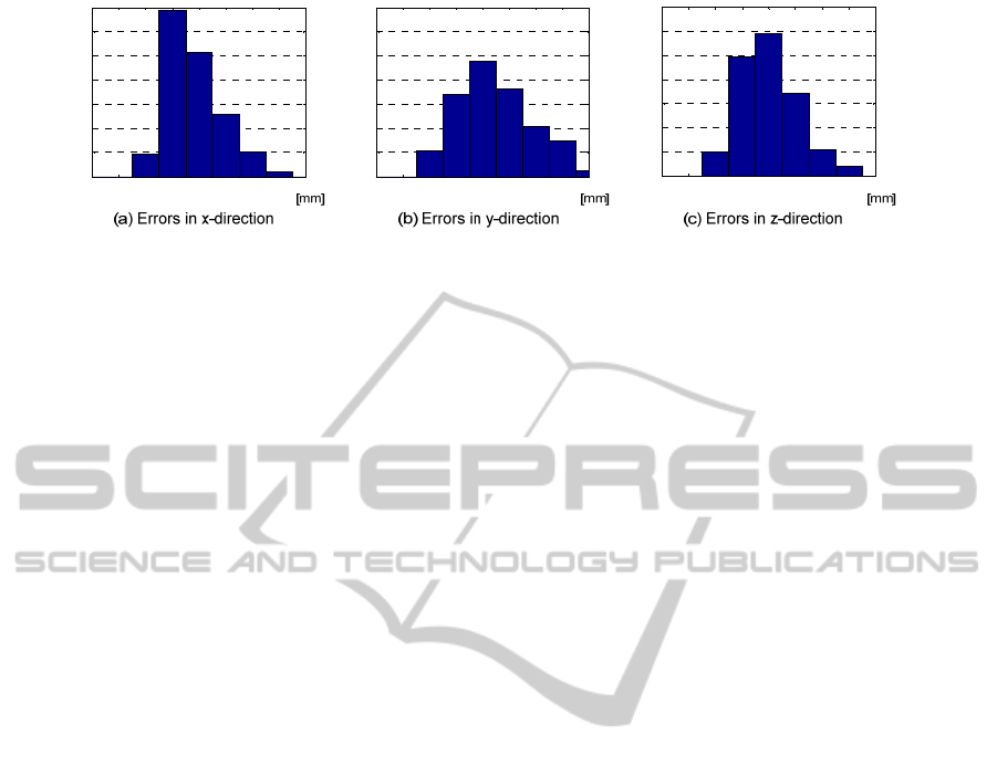
model. The histograms of the errors distribution for
the model C2 (0) show that the non-compensated
compliance errors in all directions are unbiased and
almost normally distributed.
Hence, using the developed low-order stiffness
model for the compliance error compensation gives
essential improvement of the precision for the robot-
ic based milling. It allowed us to compensate more
than 95% of deflections caused by external loading
and to guarantee the precision of about 0.2 mm un-
der the loading of 2.5 kN (it is comparable with the
robot repeatability of 0.06 mm).
5 CONCLUSION
The paper deals with the problem of the manipulator
stiffness modeling. The main attention is paid to the
elastostatic parameters identification and model re-
duction. In contrast to previous works, the manipula-
tor stiffness properties are described by the sophisti-
cated model, which takes into account the flexibili-
ties of all mechanical elements described by 6×6
stiffness matrices. This obviously yields extremely
high number of the model parameters that cannot be
CompleteStiffnessModelforaSerialRobot
199
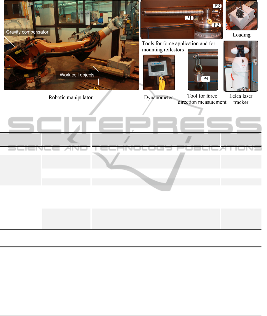
Figure 2: Experimental setup for elastostatic calibration.
Table 1: Summary of the elasto-static model reduction process for industrial robot Kuka KR-270.
Approach Step Model description
Number of pa-
rameters
Original model 6 joints +7 links (36 parameters per link) 258
Physical
M1: Symmetrisa-
tion
6 joints +7 links (21 parameters per link) 153
M2: Sparcing 6 joints +7 links (8 parameters per link) 62
M3: Aggregation 7 links (8 parameters per link) 56
Algebraic
M4a:Partitioning
M4b:Elimination
G1: Identifiable parameters – 1
G2: Non-identifiable parameters - 10
G3: Semi-identifiable parameters – 45
46
M5a:Splitting
M5b:Selection
M5c:Assigning
Selection of 25 independent parameters
from 45 semi-identifiable ones
26
Table 2: Efficiency of the compliance errors compensation using complete and reduced models.
Stiffness model
Number of
parameters
Compliance errors, mm
x-direction y-direction z-direction positional
MAX RMS MAX RMS MAX RMS MAX RMS
Deflections magnitude without compensation 2.51 1.03 3.14 1.02 8.14 1.91 8.18 4.58
Complete model C1 26 0.27 0.10 0.43 0.13 0.38 0.12 0.45 0.22
Complete model C2 30 0.28 0.10 0.45 0.14 0.32 0.11 0.49 0.21
Conventional model J1 5 1.42 0.43 1.73 0.41 0.66 0.23 1.78 0.75
Conventional model J2 9 1.42 0.42 1.73 0.42 0.49 0.19 1.76 0.73
Model C1: Complete irreducible stiffness model without gravity compensator
Model C2: Complete irreducible stiffness model with gravity compensator
Model J1: Conventional model for the manipulator with rigid links and compliant actuators, without gravity compensator
Model J2: Conventional model for the manipulator with rigid links and compliant actuators, with gravity compensator
ICINCO2014-11thInternationalConferenceonInformaticsinControl,AutomationandRobotics
200
-0.4 -0.3 -0.2 -0.1 0 0.1 0.2 0.3 0.4
0
20
40
60
80
100
120
140
-0.4 -0.3 -0.2 -0.1 0 0.1 0.2 0.3 0.4
0
20
40
60
80
100
120
140
-0.4 -0.3 -0.2 -0.1 0 0.1 0.2 0.3 0.4
0
20
40
60
80
100
120
140
Figure 3: Statistical distribution of compliance errors after compensation
identified separately. To solve the problem, physical
and algebraic model reduction methods were devel-
oped. They take into account mathematical relations
between the elements of the compliance matrices.
The advantages of the developed approach are illus-
trated by an application example that deals with
elastostatic calibration of an industrial robot used in
aerospace industry.
In future, the problem of the complete model
generation from the obtained set of parameters will
be in the focus of our attention, i.e. re-construction
of the joint compliances and 6x6 link stiffness ma-
trices from the reduced model obtained after the
identification. It is clear that this procedure requires
additional knowledge on the coupling between the
stiffness matrix elements that are induced by their
physical nature.
ACKNOWLEDGEMENTS
The authors would like to acknowledge the financial
support of the ANR, France (Project ANR-2010-
SEGI-003-02-COROUSSO) and FEDER
ROBOTEX, France.
REFERENCES
Abele, E., K. Schützer, J. Bauer and M. Pischan, 2012.
Tool path adaption based on optical measurement data
for milling with industrial robots. Prod. Eng. Res.
Devel. 6: 459-465.
Alici, G. and B. Shirinzadeh, 2005. Enhanced stiffness
modeling, identification and characterization for robot
manipulators. Robotics, IEEE Transactions on 21:
554-564.
Chen, Y., J. Gao, H. Deng, D. Zheng, X. Chen and R.
Kelly, 2013. Spatial statistical analysis and compensa-
tion of machining errors for complex surfaces. Preci-
sion Engineering 37: 203-212.
Dépincé, P. and J.-Y. Hascoët, 2006. Active integration of
tool deflection effects in end milling. Part 1. Predic-
tion of milled surfaces. International Journal of Ma-
chine Tools and Manufacture 46: 937-944.
Dumas, C., S. Caro, S. Garnier and B. Furet, 2011. Joint
stiffness identification of six-revolute industrial serial
robots. Robotics and Computer-Integrated Manufac-
turing 27: 881-888.
Karan, B. and M. Vukobratović, 1994. Calibration and
accuracy of manipulation robot models—an overview.
Mechanism and Machine Theory 29: 479-500.
Khalil, W. and E. Dombre, 2004. Modeling, identification
and control of robots. Butterworth-Heinemann.
Klimchik, A., D. Bondarenko, A. Pashkevich, S. Briot and
B. Furet, 2014. Compliance error compensation in ro-
botic-based milling. In: Informatics in control, auto-
mation and robotics. (J.-L. Ferrier, A. Bernard, O.
Gusikhin and K. Madanis, Eds.). Springer Interna-
tional Publishing, pp. 197-216.
Klimchik, A., D. Chablat and A. Pashkevich, 2014. Stiff-
ness modeling for perfect and non-perfect parallel ma-
nipulators under internal and external loadings. Mech-
anism and Machine Theory 79: 1-28.
Klimchik, A., A. Pashkevich and D. Chablat, 2013. Cad-
based approach for identification of elasto-static pa-
rameters of robotic manipulators. Finite Elements in
Analysis and Design 75: 19-30.
Klimchik, A., A. Pashkevich, D. Chablat and G. Hovland,
2013. Compliance error compensation technique for
parallel robots composed of non-perfect serial chains.
Robotics and Computer-Integrated Manufacturing 29:
385-393.
Klimchik, A., Y. Wu, G. Abba, B. Furet and A. Pash-
kevich. Robust algorithm for calibration of robotic
manipulator model. 7th IFAC Conference on Manu-
facturing Modelling, Management, and Control, 2013,
2013.
Klimchik, A., Y. Wu, C. Dumas, S. Caro, B. Furet and A.
Pashkevich. Identification of geometrical and elasto-
static parameters of heavy industrial robots. Robotics
and Automation (ICRA), 2013 IEEE International
Conference on, 6-10 May 2013, 2013.
Klimchik, A., Y. Wu, A. Pashkevich, S. Caro and B.
Furet, 2012. Optimal selection of measurement con-
figurations for stiffness model calibration of anthro-
pomorphic manipulators. Applied Mechanics and Ma-
terials 162: 161-170.
Kövecses, J. and J. Angeles, 2007. The stiffness matrix in
elastically articulated rigid-body systems. Multibody
CompleteStiffnessModelforaSerialRobot
201

System Dynamics 18: 169-184.
Lo, C.-C. and C.-Y. Hsiao, 1998. A method of tool path
compensation for repeated machining process. Interna-
tional Journal of Machine Tools and Manufacture 38:
205-213.
Lu, T.-f. and G. C. I. Lin, 1997. An on-line relative posi-
tion and orientation error calibration methodology for
workcell robot operations. Robotics and Computer-
Integrated Manufacturing 13: 89-99.
Meggiolaro, M. A., S. Dubowsky and C. Mavroidis, 2005.
Geometric and elastic error calibration of a high accu-
racy patient positioning system. Mechanism and Ma-
chine Theory 40: 415-427.
Mooring, B. W., Z. S. Roth and M. R. Driels, 1991. Fun-
damentals of manipulator calibration. Wiley New
York.
Nubiola, A. and I. A. Bonev, 2013. Absolute calibration of
an abb irb 1600 robot using a laser tracker. Robotics
and Computer-Integrated Manufacturing 29: 236-245.
Pashkevich, A. Computer-aided generation of complete
irreducible models for robotic manipulators. The 3rd
Int. Conference of Modellimg and Simulation. Univer-
sity of Technology of Troyes, France, 2001.
Roth, Z. S., B. Mooring and B. Ravani, 1987. An over-
view of robot calibration. Robotics and Automation,
IEEE Journal of 3: 377-385.
Takeda, Y., G. Shen and H. Funabashi, 2004. A dbb-based
kinematic calibration method for in-parallel actuated
mechanisms using a fourier series. Journal of Mechan-
ical Design 126: 856.
Timoshenko, S. and J. N. Goodier, 1970. Theory of elas-
ticity. McGraw-Hill, Singapore.
Wu, Y., A. Klimchik, A. Pashkevich, S. Caro and B.
Furet, 2013. Industry-oriented performance measures
for design of robot calibration experiment. In: New
trends in mechanism and machine science. Springer,
pp. 519-527.
ICINCO2014-11thInternationalConferenceonInformaticsinControl,AutomationandRobotics
202
