Interactive Visual Analysis of Lumbar Back Pain
What the Lumbar Spine Tells About Your Life
Paul Klemm
1
, Sylvia Glaßer
1
, Kai Lawonn
1
, Marko Rak
1
, Henry V¨olzke
2
, Katrin Hegenscheid
3
and Bernhard Preim
1
1
Department of Simulation and Graphics, University of Magdeburg, Magdeburg, Germany
2
Institute for Community Medicine, University of Greifswald, Greifswald, Germany
3
Institute for Diagnostic Radiology and Neuro-Radiology, University of Greifswald, Greifswald, Germany
Keywords:
Epidemiology, Interactive Visual Analysis, Classification, Multi-Modal Data.
Abstract:
Epidemiology aims to provide insight into disease causations. Hence, subject groups (cohorts) are analyzed
to correlate the subjects’ varying lifestyles, their medical properties and diseases. Recently, these cohort
studies comprise medical image data. We assess potential relations between image-derived variables of the
lumbar spine with lower back pain in a cross-sectional study. Therefore, an Interactive Visual Analysis (IVA)
framework was created and tested with 2,540 segmented lumbar spine data sets. The segmentation results are
evaluated and quantified by employing shape-describing variables, such as spine canal curvature and torsion.
We analyze mutual dependencies among shape-describing variables and non-image variables, e.g., pain indi-
cators. Therefore, we automatically train a decision tree classifier for each non-image variable. We provide
an IVA technique to compare classifiers with a decision tree quality plot. As a first result, we conclude that
image-based variables are only sufficient to describe lifestyle factors within the data. A correlation between
lumbar spine shape and lower back pain could not be found with the automatically trained classifiers. How-
ever, the presented approach is a valuable extension for the IVA of epidemiological data. Hence, relations
between non-image variables were successfully detected and described.
1 INTRODUCTION
Epidemiology is the study of dissemination, causes
and results of health-related states and events. Large
population studies, such as the Study of Health in
Pomerania (SHIP) (V¨olzke et al., 2011), gather as
much information as possible about participants to be
assessed towards different diseases. This information
is used to determine risk factors for diseases, inform
people about healthier lifestyles or to support the di-
agnosis of widespread diseases. Cohort studies are an
instrument of epidemiological research. We analyze
back pain, one of the most frequent complaints in the
Western civilization. Although the shape and consti-
tution of the spine, especially the lumbar spine, plays
an important role for back pain, an automatic clas-
sification approach for characterization of back pain
based on lumbar spine attributes is still missing.
We present an analysis of the image-derived data
from a cohort study lumbar spine dataset. We extract
possible associations between spine shape and back
pain characteristics. For this purpose, we combine
classification algorithms with data visualization tech-
niques. Then, Interactive Visual Analysis (IVA) high-
lights mutual dependencies between image-derived
data and back pain-related variables. We focus on
highlighting new correlations and trigger hypotheses
generation, rather than statistically validate complex
epidemiological correlations. Our contributions are:
• An IVA workflow for back pain analysis based on
image-derived variables of 2,240 subjects,
• The identification of lumbar spine shape proper-
ties potentially associated with back pain,
• The detection of associations between image-
based, socio-demographic and medical variables
for hypotheses generation,
• The identification of the most important variables
via classification methods using a novel decision
tree quality plot.
85
Klemm P., Glaßer S., Lawonn K., Rak M., Völzke H., Hegenscheid K. and Preim B..
Interactive Visual Analysis of Lumbar Back Pain - What the Lumbar Spine Tells About Your Life.
DOI: 10.5220/0005235500850092
In Proceedings of the 6th International Conference on Information Visualization Theory and Applications (IVAPP-2015), pages 85-92
ISBN: 978-989-758-088-8
Copyright
c
 2015 SCITEPRESS (Science and Technology Publications, Lda.)

2 EPIDEMIOLOGICAL
BACKGROUND
Epidemiological reasoning relies on a strict
statistically-driven workflow (Fletcher et al.,
2012): (1) physicians formulate hypotheses based
on observations made in their clinical practice; (2)
epidemiologists compile a list of variables depicting a
hypothesis to prove it; (3) statistical methods, such as
regression analysis, assess the correlation of selected
variables with the investigated condition. Mutually
dependent variables make this analysis challenging.
For example, the incidence rate of many diseases,
such as different cancer types increases with age
(Fletcher et al., 2012).
Challenges of Epidemiological Data Analysis.
We focus on epidemiological large scale cohort study
data. The collected data can be analyzed regarding
many diseases and conditions. Epidemiological data
are heterogenous and incomplete. For example, data
about a disease treatment only affects subjects suf-
fering from this condition. Statistical analysis has
to take missing data into account. Epidemiological
data acquisition includes a variety of techniques, such
as medical examinations, self-reported questionnaires
or genetic examinations. This yields a heterogenous
information space. Information reduction techniques
are necessary to compare these data. For example,
continuous data, such as age, is often discretized into
quantile bins for visualizing age-dependent disease
frequencies.
Modern cohort studies often comprise medical
image data. The analysis of these data is challenging.
Individual diagnosis or manual segmentation of
each body structure by radiologists is tedious, costly
and comprises little reproducibility. Segmentation
algorithms are not generally available and need to be
carefully adapted for each body structure.
Lower Back Pain. Lower back pain is one of
the most frequent complaints in the Western civiliza-
tion (Hoy et al., 2010). The exact causes as well as
particular vulnerable risk groups are unknown. Epi-
demiologists want to describe the relation between
aging and degenerative process of the spine (Szpalski
et al., 2005). They have to analyze the lumbar spine
shape as well as lifestyle factors.
3 RELATED WORK
Visual Analysis of Medical Image and Non-image
Data. In a previous work, we proposed an epidemi-
ological IVA workflow, consisting of an iterative
sequence of group selection, variable selection and
visualization (Klemm et al., 2014). Hypotheses
generation was amplified by concurrently analyzing
heterogenous variables at once using correlation
measures. (Turkay et al., 2013) derived descriptive
data metrics from image data. Their proposed
deviation plot shows distribution-specific measures
of a variable, such as skewness or inter-quantile
range, making variables comparable. This approach
aimed to trigger hypotheses generation by outlining
tendencies between these variables. A survey on
image-centric cohort studies and strategies to analyze
the resulting data is given in (Preim et al., 2015).
In a prior work, we analyzed the lumbar spine
variability of 490 subjects (Klemm et al., 2013). We
incorporated hierarchical agglomerative clustering to
derive shape groups, yielding average shape groups
and outliers. As opposed to clustering the spine
shape, we analyze the discriminative power of the
resulting data towards back pain and other non-image
variables in this work.
Visual Analysis of Heterogenous Non-image
Data. (Zhang et al., 2012) analyzed subject groups
in a web-based linked view system. The resulting
decision rules aim to categorize new subjects as
they are added to the data. They defined a cohort
as variable-divided subject group, differing from
the epidemiological understanding of the term. The
described method lacks details about handling of
missing data, the definition of similarity or the choice
of the statistical measures. Generalized Pairs Plots
(
GPLOMs ) visualize heterogenous variables in a plot
matrix (Emerson et al., 2013). The plot depends on
the type of variables, which are visualized pairwise.
GPLOMs provide an overview, but take up much
screen space and are therefore only suitable for a few
variables at once (see example in Fig. 2).
Decision Rule-driven Analysis of Medical Data.
Closest to ours is the work of (Glaßer et al., 2013)
and (Niemann et al., 2014). Both used decision trees
for their analyses. Decision trees are easily readable
and are frequently used for classifying medical data.
(Glaßer et al., 2013) used variables derived from
DCE-MRI data capturing the perfusion in tumorous
tissue. To classify breast tumors, they trained a
decision-tree classifier, concluding that the extracted
kinetic and morphological variables alone are not
sufficient for tumor type classification. (Niemann
et al., 2014) assessed risk factors for hepatic steatosis
(fatty liver disease) using decision trees. Their inter-
active data mining tool can analyze association rules
IVAPP2015-InternationalConferenceonInformationVisualizationTheoryandApplications
86

and highlights relations. We combine both ideas by
validatingthe significance of image-derivedvariables.
Unique in our work is the combination of clas-
sification techniques with an IVA approach by
observing interesting variable relations in the context
of image-derived variables using multiple decision
trees for one visualization. We abstract the decision
tree results similar to (Turkay et al., 2013), making
them comparable in an overview visualization.
4 THE LUMBAR SPINE DATA SET
Our work is based on a data set compiled by Epi-
demiologists with a wide range of variables possibly
correlating with lumbar back pain, comprising non-
image and image-derived data for 3,234 subjects.
Non-image Data. The non-image variables
range from somatometric variables describing body
measures to medical examinations, such as laboratory
tests as well as lifestyle factors, e.g., sporting activity
or nutrition. The data set comprises 134 variables:
• 21 metric variables, describing somatometric vari-
ables and markers retrieved from blood analysis.
• 113 categorical variables divided into 43 dichoto-
mous (binary) variables, mostly indicating the
presence of a disease, e.g., pancreatitis or high
blood pressure, and 70 variables with more than
two levels, indicating pain levels, nutrition and so-
cial factors, such as marital or retirement status.
All categorical variables are converted into binary
dummy variables, indicating the presence or absence
of a categorical variable manifestation. For example,
a pain indicator variable ranging from 1 - no pain to
4 - large pain is subdivided into four dichotomous
variables to determine, which manifestation can be
described best using the image-based variables.
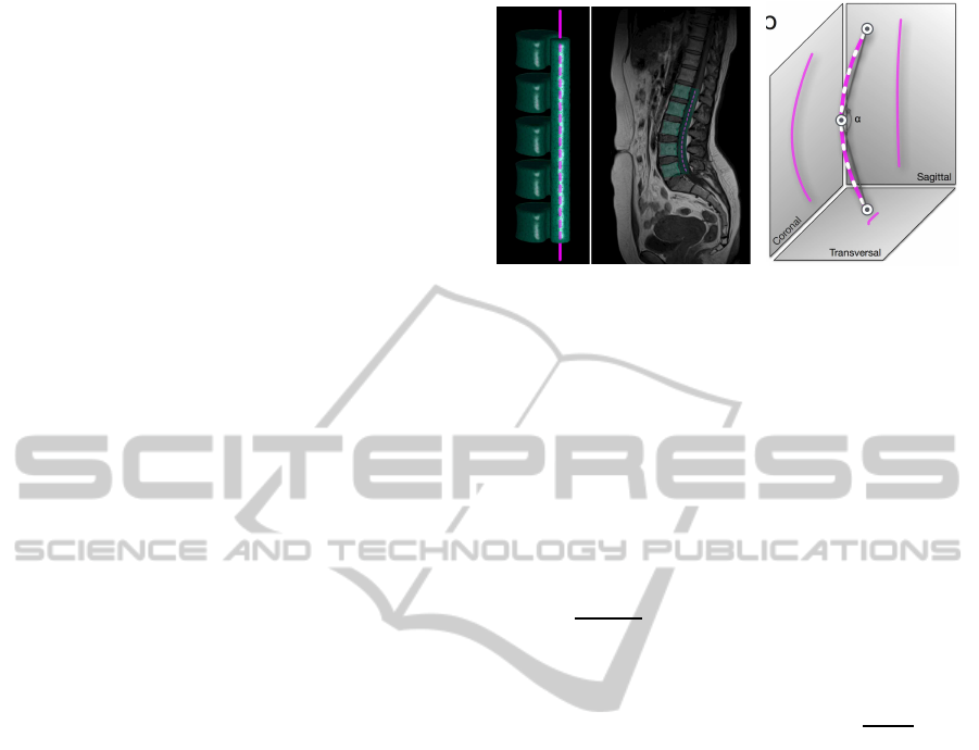
Image-derived Data. Magnetic Resonance Imaging
(MRI) scans were obtained for each subject (Hegen-
scheid et al., 2013). A hierarchical finite element
method was used to detect the lumbar spine in the
MRI data (Rak et al., 2013). The tetrahedron-based
finite element model (Fig. 1 a) captures information
about the lumbar spine canal shape and the position
of the L1-L5 vertebrae. The detection fails for
several subjects due to imaging artifacts or strongly
deformed spines, yielding models for 2, 540 out of
3, 234 subjects. The detection model depicts the
vertebrae positions, spine canal curvature, but lacks
detailed information about their volume. In (Klemm
Transversal
Sagittal
Coronal
a b
α
L1
L2
L3
L4
L5
Figure 1: (a) Finite element model (FEM) of the lumbar
spine (left), capturing the L1-L5 vertebrae and the lumbar
spine canal (right). The purple dashed line describes the
lumbar spine canal centerline with 92 points. (b) We ex-
tract the weighted sum of curvature and torsion for all 92
points (white dashes) and the curvature angle (α) for each
projection axis to assess their information gain.
et al., 2013), we extracted a centerline representation
of the lumbar spine canal from the detection model
(Fig. 1 a). Using the Frenet frame, we calculated the
following metrics from the model (Fig. 1 b):
• Mean Curvature is defined as the average cur-
vature of all points describing the centerline:
∑
I
i=1
curvature
i
I
. We refer to the mean curvature as
curvature.
• Mean Torsion (deviation of a curve from its cur-
rent course) is defined as the average torsion of all
points describing the centerline:
∑
I
i=1
torsion
i
I
. We
refer to the mean torsion as torsion.
• Curvature angle α is the angle defined by the
middle point of the spine canal centerline as ver-
tex and the line connecting middle point and
top/bottom point as sides.
These metrics are also extracted in the sagittal, coro-
nal and transversal projection of the model, yielding
9 image-derived variables. In the next section, we
present the experimentswe conducted to assess the in-
fluence of the lumbar spine shape to lower back pain.
5 EXPERIMENTS AND
PRELIMINARY RESULTS
In this section, the image-derived variables are ana-
lyzed towards the dichotomous back pain indicator
using a
GPLOM and all non-image variables using
heterogenous correlations. Spine shape is influenced
by several somatometric variables. Larger people
also have a longer spine with a straighter shape. High
body weight increases the spine load, resulting in a
bent shape. To assess their influence, we take them
into account when spine curvature and torsion are
InteractiveVisualAnalysisofLumbarBackPain-WhattheLumbarSpineTellsAboutYourLife
87

Mean Curvature
Mean Torsion
Mean Curvature
Coronal
Mean Curvature
Sagittal
Mean Curvature
Transverse
Curvature Angle
Curvature Angle
Coronal
Curvature Angle
Sagittal
Curvature Angle
Transverse
Back Pain
Yes
No
Cor: -0.0103
Yes: -0.015
No: -0.042
Cor: 0.605
Yes: 0.607
No: 0.603
Cor: 0.99
Yes: 0.989
No: 0.991
Cor: -0.0379
Yes: -0.247
No: -0.0733
Cor: -0.0888
Yes: -0.887
No: -0.889
Cor: -0.311
Yes: -0.336
No: -0.269
Cor: -0.872
Yes: -0.871
No: -0.875
Cor: -0.2
Yes: -0.205
No: -0.194
Cor: 0.0024
Yes: 0.0281
No: 0.0477
Cor: -0.0129
Yes: -0.0113
No: -0.0157
Cor: 0.0049
Yes: 0.0005
No: 0.0145
Cor: 0.0047
Yes: 0.0056
No: 0.0035
Cor: -0.0151
Yes: 0.0211
No: -0.069
Cor: 0.0066
Yes: 0.0030
No: 0.0118
Cor: 0.0216
Yes: 0.0294
No: 0.0084
Cor: 0.491
Yes: 0.489
No: 0.495
Cor: -0.0551
Yes: -0.0532
No: -0.0667
Cor: -0.421
Yes: -0.417
No: -0.429
Cor: -0.75
Yes: -0.751
No: -0.747
Cor: -0.358
Yes: -0.353
No: -0.368
Cor: -0.0592
Yes: -0.0724
No: -0.0373
Cor: -0.0319
Yes: -0.0176
No: -0.0689
Cor: -0.901
Yes: -0.902
No: -0.9
Cor: -0.221
Yes: -0.247
No: -0.179
Cor: -0.896
Yes: -0.896
No: -0.896
Cor: -0.21
Yes: -0.214
No: -0.207
Cor: 0.0215
Yes: 0.0071
No: 0.0672
Cor: 0.0353
Yes: 0.0435
No: 0.0225
Cor: 0.0184
Yes: 0.00355
No: 0.055
Cor: 0.0181
Yes: 0.0267
No: -0.0058
Cor: 0.217
Yes: 0.235
No: 0.189
Cor: 0.995
Yes: 0.994
No: 0.995
Cor: 0.387
Yes: 0.383
No: 0.397
Cor: 0.134
Yes: 0.15
No: 0.108
Cor: 0.0439
Yes: 0.0607
No: 0.0145
Cor: 0.392
Yes: 0.386
No: 0.405
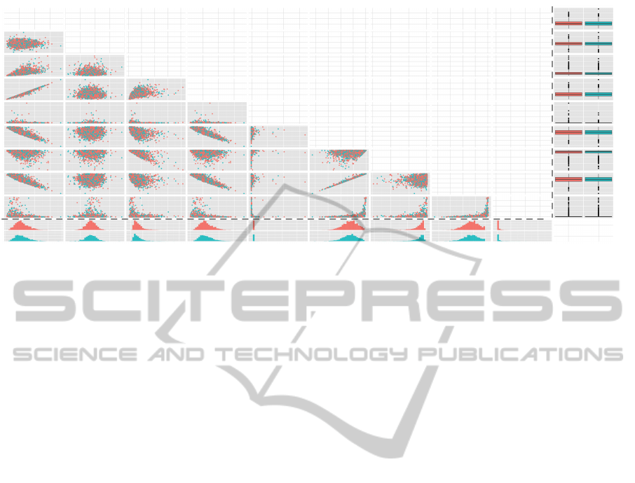
Figure 2: A GPLOM of all image-derived variables colored by presence (red) or absence (turquoise) of back pain. Pairwise
combinations of image-derived variables are visualized via scatter plots on the left of the matrix diagonal. Their correlation
with back pain is denoted to the right of the matrix diagonal. The box plots (right) and histograms (bottom) display the
distribution of each image variable encoded with back pain. No correlations with back pain can be identified in this plot.
correlated with non-image variables. Discretizing
metric variables using quartiles avoids outlier groups.
GPLOM Analysis. As first experiment we cor-
related the shape variable with the dichotomous back
pain indicator using a GPLOM (Fig. 2). The metric
image-derived variables are pairwise visualized using
scatter plots on the left side of the matrix diagonal.
The combination of the image variables with back
pain is visualized as histogram in the last row and
as box plot in the last column. The projections to
the transversal planes attract attention as they have
many outliers. We conclude that curvature is not as
reliable on the transversal plane as it is on the other
planes, which was also confirmed through a principal
component analysis (see supplementary material
at ivapp15.dnsalias.com). The
GPLOM shows similar
distributions of subjects with or without back pain
with respect to the shape variables in all sub-plots.
Heterogenous Correlations. We then expanded our
focus on correlations of image-derived variables with
all other non-image variables. Different correlation
metrics depending on the type of the individual
variables are used to derive correlations between
all variables in the data set. The method uses the
Pearson product-moment for two continuous vari-
ables, polyserial correlation for one continuous and
one categorical variable and polychoric correlations
for two categorical variables. All values are scaled
between
0 - no correlation and 1 - perfect
correlation
. Some variables are too sparse for
calculating correlations, for example treatment of
diabetes, or medication against high blood pressure
are omitted, since they are not statistically resilient.
We display the resulting contingency matrix using
a heat map, encoding correlation values with color
brightness with white for 0 and dark blue for 1. We
calculated the contingency matrix for all size groups
and searched for correlations between image- and
non-image variables. The resulting contingency
matrices show no strong correlation with image vari-
ables (see experiments page at ivapp15.dnsalias.com).
Only weak correlations could be found for mean
curvature with gender (0.42), body size (0.39) and
number of born children (0.29). One surprising result
was the small correlation of torsion with Parkinson’s
disease (0.24). Other than that, torsion correlated
with almost no variables (values between 0 and 0.05).
These observations brought us to the decision to
incorporate classification techniques to assess the in-
fluence of the image-derived variables.
6 INTERACTIVE DECISION
TREE QUALITY PLOT
As described before, correlation coefficients fail
to infer back pain status based on lumbar spine
canal curvature and torsion. We rely on predic-
tive classification to obtain a complex rule set on
how combinations of the image-variables explain
non-image variables. Decision trees are used to
create predictive models. These models are built
w.r.t. all input variables and capture more complex
relationships than correlation coefficients. Leafs
of a decision tree represent class labels, branches
represent variable conjunctions leading to the class
IVAPP2015-InternationalConferenceonInformationVisualizationTheoryandApplications
88

labels. Decision trees are easy to understand and to
read. Too many branches impose overfitting to the
data (Mitchell, 1997).
Creating Decision Trees. We use the C4.5 al-
gorithm, which builds decision trees based on
information entropy. Categorical attributes with
more levels are biased with more information gain
in a decision tree (Deng et al., 2011). Creating a
dummy variable by converting each manifestation of
a categorical variable into a dichotomous variable
bypasses this problem. In the following analysis, we
strongly focus on the complexity of decision trees
and the classification accuracy.
We have to create a decision tree for every
non-image variable to analyze which one can be
explained by image-derived variables. Since we have
134 non-image variables, the calculation yields the
same amount of trees. Further subdivision, e.g., by
quantiles of body mass index, increases the number
to 402 trees. We have to abstract the results of the
classification to keep the mental effort of interpreting
the data low.
Decision Tree Quality Plot. We follow the Vi-
sual Analytics mantra of analyzing first, show the
important and analyze further (Keim et al., 2008).
A first analysis step was performed by applying the
classification algorithm to the data. The optimal
classification uses a few rules to precisely describe
the target variable. Therefore, we are interested
in small trees with a low classification error. The
two measures form the axes for a scatter plot of the
classification results. This decision tree quality plot
is our central element for the interactive analysis of
decision trees.
The Error Term. Calculating the mean classification
error is imprecise for non-uniform distributions. For
example, if a variable indicating a disease is negative
for 90% of the subjects and the classifier simply
assigns all subjects to not ill, we get a mean error of
10%, even though it is very imprecise. Based on this
we use a summary error based on the weighted mean,
which incorporates the discriminative power of each
manifestation and is denoted as follows:
totalError = 1−
M
∑
m=1
correctlyClassified
m
M ·N
m
(1)
M represents the set of manifestations of each
variable. N
m
denotes the number of subjects in
manifestation m. The error represents the share of
incorrect classifications and denotes perfect classifi-
cation with 0 and always wrong with 1. We display
results below 0.5 in the visualization, a value below
0.25 represents a good classification. It allows for
comparability of error rates between variables with
different manifestation count.
Attribute Mapping. The scatter plot axes are
defined by tree size and the previously described
error metric. This allows us to visualize a multitude
of classification results in one plot. Classification
and comparison of variables for subject groups
(e.g., male and female subjects) in one plot can be
achieved by color coding group affiliation on the
data points. Many variables are sparse, such as
medication of diabetes or reason of early retirement.
The classification algorithm may produce higher
accuracy for variables with less subjects due to the
small sample size, making these results less reliable.
Therefore, we provide a way to adjust the minimal
number of subjects for each variable using a slider.
The initial value is empirically set to 100, marking a
good tradeoff between sparse variables and statistical
informative value. Furthermore, we map the number
of subjects associated with a variable to the diameter
in the decision tree quality plot. This allows instant
reliability assessment of the result. We apply a
square root scale for the tree size axis to highlight
decision trees with few decision rules. Outlier results
with large decision trees would otherwise distort the
resulting plot.
Decision Tree Quality Plot Interaction. The
visualization provides a good overview of the clas-
sification results. Details-on-demand are displayed
by clicking on an entry in the visualization, which
then displays the corresponding decision tree in
detail. This allows to sequentially analyze the
classifications. We provide controls for adjusting the
maximum classification error and minimum subject
count for a variable. This gives the user control to
abstract or refine the displayed information. The
subject subdivision is controlled by the selection
of variables, such as gender or employment status.
Metric variables, such as body size, are discretized
using their quantiles. This allows to assess the
influence of a variable to the classification process.
Implementation. All analyses are available at
ivapp15.dnsalias.com and are carried out using
R , a
widely used programming language for statistical
calculations and visualizations. The interactive
visualizations are realized using the
ggvis
1
package.
The web-based approach allows for quick exchange
with our collaborating epidemiological experts. They
can use the technique without installing any software.
1
Developed by RStudio, Inc;
ggvis.rstudio.com
InteractiveVisualAnalysisofLumbarBackPain-WhattheLumbarSpineTellsAboutYourLife
89

a
Error Rate
Tree Size
2
√
Error Rate
Tree Size
2
√
!"# !"$ %"# %"$ &"# &"$ $"# $"$ '"# '"$ ("#
#"%!
#"%&
#"%'
#"%)
#"&#
#"&!
#"&&
#"&'
#"&)
*+,-./0%120'&3
+4*564+7.089845:87:87;;
*+,-./0((2!#!3
4<:=+:+549*7<*7>-.0898?7+;@85=87;65*:8A7+;@
B>-./'&21#3
C+>C8D;55A8E=-**<=-96-A+F7:+54
D;57:+4>.089845:87:87;;
=7A+7:+4>9D7FGE7+4.0898H5
!"#$"%
!" #" $" %" &" '" ("
")$#
")$%
")$'
")$*
")%"
")%#
")%%
")%'
")%*
+,-.,/
.012,3,453/,136,-3
708792:;;.9</,44=/,56,.0>130;-
!"#$
c
Error Rate
Tree Size
2
√
Error Rate
Tree Size
2
√
!"# !"$ %"# %"$ &"# &"$ $"# $"$ '"# '"$ ("# ("$ )"#
#"!)
#"%#
#"%!
#"%&
#"%'
#"%)
#"&#
#"&!
#"&&
#"&'
#"&)
*+,-./0%120'&3
4-56-7
4-56-7
4-56-7
896:.;<=.>-7?-5=./%&"02$!"(3
@A-./!02&%")3
896:.;<=.>-7?-5=./#"%2!!"13
B-+AC=./&0"$2(#"$3
D+E+5A.B+=C.><7=5-7
?9D6.C:>-7*-5*+=+E-.0FGF59=F<=F<DD
><+5.D-A*.#
4-56-7
896:.;<=.>-7?-5=./#"%2!!"13
=C:79+6.596HD-*
I9+5=.D+J8.><+5.&FGF*=795A
=-5*+95.0FGF59=F<=F<DD
5H=7+=+95.*<H*<A-.0FGFK<+D:F97F<DJ9*=F6<+D:
*+,-./0%120'&3
L5?7-<*-6.8D996.D+>+6
5-?M.*C9HD6-7.><+5.&FGF*=795A
5-?M.*C9HD6-7.><+5.%FGFJ96-7<=-D:
8<?M.><+5.+56H?-6.*9?+<D.>798D-J*.!FGFC<76D:
!"#$%&"'(%)%*"+'
!"#$%#%&!'()*+
! "# "! $# $! %# %! &# &! !# !! '#
#($&
#($'
#($)
#(%#
#(%$
#(%&
#(%'
#(%)
#(&#
#(&$
#(&&
#(&'
#(&)
#(!#
*+,-./*0/,1-.23456+
*+,-./*0/,1-.23456+
.57,
8,61,0
*+,-./*0/,1-.23456+
8,61,0
8,61,0
9*56-:*./-;-1*<.
=5+=>?:331>90,..@0,-2,15A*/536
.57,
=5+=>?:331>90,..@0,-2,15A*/536
:5B56+-C5/=-9*0/6,0
8,61,0
*:0,*1<-2,6./0@*:-9,0531
D+,
/=<0351-631@:,.
C,5+=/
EFG-H
F6A0,*.,1-?:331-:5951
9*56-:,+.
6@/05/536-I@,.:5
*?13256*:-9*56
6@/05/536-A*4,
!"#$#%&'$#(
!&'$#%&#$'(
!&#$'%)*$+(
!)*$+%',(
BMI
b
Error Rate
Tree Size
2
√
Error Rate
Tree Size
2
√
!"# !"$ %"# %"$ &"# &"$ $"# $"$ '"#
#"!&
#"!'
#"!(
#"%#
#"%!
#"%&
#"%'
#"%(
#"&#
#"&!
#"&&
#"&'
#"&(
)*+,-./%01/'&2
34*567,8)-!
9,4:*5,))-/;6;5<=;4=;477
>8,-.'&10#2
)*+,-./??1!#!2
=,5)*<5-/;6;5<=;4=;477
@<7A69B3,C),5)*=*:,-/;6;5<=;4=;477
!"#$%&'"%()*)+,
! "# "! $# $! %# %! &# &! !#
#'$&
#'$(
#'$)
#'%#
#'%$
#'%&
#'%(
#'%)
#'&#
#'&$
#'&&
#'&(
#'&)
*+,-./0+.123245
67-84/6./-3845192:7
0270;<=113;,.-44>.-85-32?6/21:
06.38@1.92:7
!"#
!"#$
%$!"#$
Gender
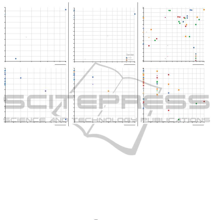
Figure 3: Decision tree quality plot of all classification results. The x-axis shows the number of decisions of the underlying
model, the y-axis the classification error (see Section 6). The upper plot shows the results for all variables, either metrics
expressed via their quantiles, or categorical. The lower plot displays the dummy variables derived from the original variables.
Group affiliation of a data point is color coded: no group (a), subdivision into male and female subjects (b) and quartiles of
Body Mass Index (BMI) (c). The number of subjects represented in a variable is denoted using the dot diameter. We only
display variables with an error below 0.5, results above this threshold are dismissed. The interactive plot (see supplemental
material) has clickable data points, displaying the corresponding decision tree in a tool tip. Results of high interest are located
close to the axis origins.
7 RESULTS
In this section, we show which non-image variables
can be explained using the 9 image derived variables.
We create subject groups to assess the influence
of variables affecting the lumbar spine shape. The
groups are: all subjects; males and females; and a
subdivision by Body Mass Index quantiles (BMI =
m
l
2
where m is the body mass in kilogram and l is the
body size in meter), yielding the groups (17, 24.7]
(24.7, 27.4] (27.4, 30.5] (30.5, 48]. We plotted
each group twice. The first plot shows all origi-
nal variables, the second all categorical variables
transformed into dichotomous dummy variables.
The shown mutual dependencies aim to amplify
hypotheses generation. Dedicated statistical analysis
of these results solely focussed on epidemiological
research is not the scope of this paper. The resulting
plots can be seen in Figure 3.
All Variables. The majority of non-image vari-
ables cannot be automatically classified based on the
image-variables. This is reflected in the large amount
of variables classified with an error above 0.6.
None of the pain indicators can be reliably
described using the image-based variables. The only
variable reliably classified in this group is gender,
which can be described with an error of 0.31 using 7
rules and incorporates only curvature- and curvature
angle-related variables. The distinctness lies in the
average difference in body size between male and
female subjects. Medication for high blood pressure
is classified for 1,058 subjects with an error of 0.47
solely based on coronal mean curvature. A high
share of medicated subjects were correctly classified
(796 of 1, 058). The majority of non-medicated
subjects are false-positive classified (262 of 1, 058),
yielding a poor quality of the classifier w.r.t. epidemi-
ological research. The four body size groups could
be described with an error of 0.48, but the decision
tree comprises 71 rules and imposes overfitting. The
dummy variable analysis yields a result similar to the
blood pressure medication. Variables, such as subject
size 139-164 cm, between 64 and 90 years of age or
IVAPP2015-InternationalConferenceonInformationVisualizationTheoryandApplications
90

nutrition-related variables are dominantly populated
by one manifestation. The classifier neglects the
other groups and yields an error below 0.5.
Gender Groups. Classifications using groups
divided by gender do not produce satisfying results.
Only hypothyroidism could be described for male
subjects with an error of 0.24 for 110 subjects using
the mean curvature and curvature angle. Since
there are only 30 male subjects diagnosed with
hypothyroidism, the statistical power of the result
is reduced. The dummy variable analysis showed
that female subjects of 139-164 cm body size could
be discriminated using the mean curvature and
curvature angle, with an error of 0.38.
Body Mass Index Groups. Gender could be
classified for each BMI group using mean curvature
and curvature angle. The error varies between 0.31
(BMI of 30.5 − 48, 4 decision rules) to 0.39 (BMI
of 24.7 − 27.4, 5 decision rules). The starting age
of smoking could be described well with an error
between 0.25 and 0.32 for all BMI groups except
for subjects with a BMI of 30.5−48. The result is
overfitted to the data due to tree sizes between 14
and 16. Some variables, such as body size, can be
described with an error of 0.3 to 0.36 using large
decision trees with over 20 rules. Using mostly mean
curvature and curvature angle, the leg pain level can
be described using 14 rules with an error of 0.46
for obese subjects (BMI higher than 30). This result
also imposes overfitting. Subjects experiencing pain
in the last seven days can also be described for this
group using the same variables with a tree consisting
of 8 rules and an error of 0.35. Obese subjects are
prone to back and leg pain due to a more stressed
lumbar spine. The stress-induced spine deformation
seems to directly influence the pain levels for these
subjects. The dummy variable analysis shows many
results using a decision tree with one rule based on
mean curvature or curvature angle with an error
between 0.35 and 0.47.
8 SUMMARY & CONCLUSION
We provide a method for comparative analysis of de-
cision trees independent of the variable manifestation
count using a novel decision tree quality plot. We
applied the method to gain insight into the predic-
tive power of 9 image-derived variables for 134 non-
image variables with focus on back pain. The analysis
was performed for subject groups of gender, BMI and
body size to assess their influence on the lumbar spine
shape.
The methods presented herein may be applied to
comprehensive epidemiological data sets to inves-
tigate mutual dependencies among variables and to
generate hypotheses on potential associations and
subgroups. These hypotheses, however, have to be
substantiated by dedicated statistical analyses and
replication in independent cohorts.
Predictive Power of Image-Derived Variables.
The presented results indicate that torsion, curvature
and curvature angle of the lumbar spine at the pre-
sented precision are not sufficient to describe lumbar
back pain in the SHIP data set. Our method allows
to assess their discriminative power, which is largely
limited to separating male and female subjects, nutri-
tion variables, as well as different disease indicators.
The C4.5 algorithm proved to be an effective tool for
evaluating a set of derived metrics regarding their
suitability to classify non-image variables. Over-
fitting to the data indicated by complex decision trees
has to be taken into account as well. The presented
method only captures linear relationships between
variables. To take more complex associations into
account, methods such as regression analysis have to
be incorporated.
Applicability. Methods supporting hypotheses
generation based on image information are new
to the application domain. They are an addition
to the standard epidemiological workflow as they
highlight new and possibly unknown relationships.
Classification methods based on decision trees have
proven to be useful for assessing the discriminative
power of a variable set. Their ability to consider vari-
able combinations makes them more powerful than
correlation coefficients calculated for each variable.
This advantage comes with a much more complex
output, the results are more challenging to assess and
to abstract. Our method to plot derived metrics and
custom-tailored error measures proved to be effective.
Huge result spaces could be navigated fast using our
decision tree quality plot. Therefore, the method is
applicable not only for deriving information based on
image data, but on all potential target variables.
Future Work. We will focus on more precise
models for extracting measures. Dented vertebrae
indicate pathological deformation, and can be cap-
tured by segmenting the top and bottom point of
each vertebra center. Spine canal thickness indicates
signs of herniated disc disease and is also of interest.
We aim to include the method into existing visual
analytics methods designed for analyzing shape infor-
InteractiveVisualAnalysisofLumbarBackPain-WhattheLumbarSpineTellsAboutYourLife
91

mation for epidemiological data (Klemm et al., 2014).
Outlook. Combining the power of statistical
analyses, visual analytics and classification tech-
niques is essential for analyzing increasingly complex
heterogenous population data. These methods do
not aim to replace the traditional epidemiological
workflow, but rather complement the weak points of
standard statistical methods. Our method provides
a novel way to gain insight into these complex data
sets and amplifies hypotheses generation.
ACKNOWLEDGEMENTS
SHIP is part of the Community Medicine Research net of
the University of Greifswald, Germany, which is funded
by the Federal Ministry of Education and Research (grant
no. 03ZIK012), the Ministry of Cultural Affairs as well as
the Social Ministry of the Federal State of Mecklenburg-
West Pomerania. Whole-body MR imaging was supported
by a joint grant from Siemens Healthcare, Erlangen, Ger-
many and the Federal State of Mecklenburg-Vorpommern.
The University of Greifswald is a member of the Centre of
Knowledge Interchange program of the Siemens AG. This
work was supported by the DFG Priority Program 1335:
Scalable Visual Analytics. This work was supported by the
federal state of Saxony-Anhalt under grant number ’I 60’
within the Forschungscampus STIMULATE.
REFERENCES
Deng, H., Runger, G., and Tuv, E. (2011). Bias of im-
portance measures for multi-valued attributes and so-
lutions. In Artificial Neural Networks and Machine
Learning–ICANN 2011, pages 293–300. Springer.
Emerson, J. W., Green, W. A., Schloerke, B., Crowley, J.,
Cook, D., Hofmann, H., and Wickham, H. (2013).
The generalized pairs plot. Journal of Computational
and Graphical Statistics, 22(1):79–91.
Fletcher, R. H., Fletcher, S. W., and Fletcher, G. S. (2012).
Clinical epidemiology: the essentials. Lippincott
Williams & Wilkins.
Glaßer, S., Niemann, U., Preim, B., and Spiliopoulou, M.
(2013). Can we Distinguish Between Benign and Ma-
lignant Breast Tumors in DCE-MRI by Studying a Tu-
mors Most Suspect Region Only? In Proc. of Sympo-
sium on Computer-Based Medical Systems (CBMS),
pages 59–64.
Hegenscheid, K., Seipel, R., Schmidt, C. O., V¨olzke, H.,
K¨uhn, J.-P., Biffar, R., Kroemer, H. K., Hosten, N.,
and Puls, R. (2013). Potentially relevant incidental
findings on research whole-body MRI in the general
adult population: frequencies and management. Eu-
ropean Radiology, 23(3):816–826.
Hoy, D., Brooks, P., Blyth, F., and Buchbinder, R. (2010).
The epidemiology of low back pain. Best Practice and
Research Clinical Rheumatology, 24(6):769 – 781.
Keim, D. A., Mansmann, F., Schneidewind, J., Thomas, J.,
and Ziegler, H. (2008). Visual analytics: Scope and
challenges. Springer.
Klemm, P., Lawonn, K., Rak, M., Preim, B., T¨onnies, K.,
Hegenscheid, K., V¨olzke, H., and Oeltze, S. (2013).
Visualization and Analysis of Lumbar Spine Canal
Variability in Cohort Study Data. In Proc. of Vision,
Modeling, Visualization 2013, pages 121–128.
Klemm, P., Oeltze, S., Lawonn, K., Hegenscheid, K.,
V¨olzke, H., and Preim, B. (2014). Interactive vi-
sual analysis of image-centric cohort study data.
IEEE Trans. on Visualization and Computer Graph-
ics, 20(12):1673–1682.
Mitchell, T. M. (1997). Machine learning. 1997. Burr
Ridge, IL: McGraw Hill, 45.
Niemann, U., V¨olzke, H., K¨uhn, J.-P., and Spiliopoulou,
M. (2014). Learning and inspecting classification
rules from longitudinal epidemiological data to iden-
tify predictive features on hepatic steatosis. Expert
Systems with Applications.
Preim, B., Klemm, P., Hauser, H., Hegenscheid, K., Oeltze,
S., Toennies, K., and V¨olzke, H. (2015). Visual Ana-
lytics of Image-Centric Cohort Studies in Epidemiol-
ogy, chapter Visualization in Medicine and Life Sci-
ences III, page in print. Springer.
Rak, M., Engel, K., and Toennies, K. (2013). Closed-form
hierarchical finite element models for part-based ob-
ject detection. In Proc. of Vision, Modeling, Visual-
ization 2013, pages 137–144.
Szpalski, M., Gunzburg, R., M´elot, C., and Aebi, M. (2005).
The aging of the population: a growing concern for
spine care in the twenty-first century. In The Aging
Spine, pages 1–3. Springer.
Turkay, C., Lundervold, A., Lundervold, A. J., and Hauser,
H. (2013). Hypothesis generation by interactive vi-
sual exploration of heterogeneous medical data. In
Human-Computer Interaction and Knowledge Dis-
covery in Complex, Unstructured, Big Data, pages 1–
12. Springer.
V¨olzke, H., Alte, D., Schmidt, C., et al. (2011). Cohort Pro-
file: The Study of Health in Pomerania. International
Journal of Epidemiology, 40(2):294–307.
Zhang, Z., Gotz, D., and Perer, A. (2012). Interactive vi-
sual patient cohort analysis. In Proc. of IEEE VisWeek
Workshop on Visual Analytics in Health Care.
IVAPP2015-InternationalConferenceonInformationVisualizationTheoryandApplications
92