
Prediction-aided Radio-interferometric Object Tracking
Gergely Zachár and Gyula Simon
Department of Computer Science and Systems Technology, University of Pannonia, Veszprém, Hungary
Keywords: Sensor Network, Localization, Tracking, Radio-interferometry, Prediction.
Abstract: In this paper a novel robust radio-interferometric object tracking method is proposed. The system contains
fixed infrastructure transmitter nodes generating interference signals, the phases of which are measured by
the tracked receivers and other fixed infrastructure nodes. From the measured phase values a confidence
map is computed, which is used to generate the track of the moving receivers. The proposed method
enhances the track estimation by an adaptive evaluation method of the confidence map, and also provides
more robust estimation by allowing bad or missing measurements, which are tolerated by predictions
extracted from the evolution of the confidence map in time. The performance of the proposed system is
illustrated by real measurements.
1 INTRODUCTION
Object localization and tracking, where the goal is to
determine the location of a target of interests, is a
key service in many applications. Several different
technologies have been proposed, the most notables
being the image-, acoustic-, and RF-based solutions.
Image-based techniques identify image features
in consecutive video frames and thus can localize
and track objects (e.g. Se, 2001). Low-cost solutions
use special graphical markers to aid localization (e.g.
in museums (Mulloni, 2009). Other systems use a
large database of pictures to determine the current
location by comparing the picture taken at the
unknown location to the pictures stored in the
database (Kai, 2009).
Acoustic localization methods mainly use
triangulation based on ranging, which is performed
by measuring the time of flight of sound (Peng,
2007).
The most widespread RF-based solution is GPS,
which utilizes the time of flight of electromagnetic
signals emitted from several satellites to triangulate
the position of a receiver. GPS can be used mainly in
outdoors applications, where the line of sight to
some satellites can be provided. Indoors applications
also use RF-based solutions, either using received
signal strength (RSSI) or the time of flight. Since
RSSI cannot be used reliably for ranging (i.e. for
distant measurement), RSSI-based solutions often
use reference maps, measured during system setup
(Au, 2012). RF ranging-based solutions measure the
time of flight of RF signals, using more
sophisticated hardware (Lanzisera 2011). A
completely different approach was proposed in
(Maroti, 2005) to avoid high frequency processing,
based on radio interferometric phase measurements.
The robustness and the processing speed of the radio
interferometric localization were improved in (Dil,
2011) with a stochastic approach. For real-time
interferometric tracking a confidence map-based
approach was proposed by (Zachár, 2014), which is
either able to follow the trajectory of an object if its
original position is known, or it can determine the
full track of a moving object retrospectively if the
object has covered a sufficiently large trajectory.
In this paper a novel object tracking method will
be proposed, which utilizes radio-interferometric
phase measurements and confidence maps, similar to
(Zachár, 2014), but enhances the robustness and
quality of the position estimation. The main
contributions of the paper are the following:
For the evaluation of peaks in the confidence
map a dynamic threshold value is proposed,
which is based on the statistical properties of the
confidence map. This solution provides more
robust estimates in real situations, when the
environment changes (e.g. people are moving
around the tracked object).
Missing or bad measurements are tolerated by a
novel prediction method, which examines the
evolution of the confidence map in time and
161
Zachár G. and Simon G..
Prediction-aided Radio-interferometric Object Tracking.
DOI: 10.5220/0005241501610168
In Proceedings of the 4th International Conference on Sensor Networks (SENSORNETS-2015), pages 161-168
ISBN: 978-989-758-086-4
Copyright
c
2015 SCITEPRESS (Science and Technology Publications, Lda.)

extracts prediction information from it.
The proposed method provides more robust and
more accurate estimates when bad measurements are
present or measurements are temporarily missing.
The complexity of the proposed algorithm is
moderate thus it can be implemented in real time on
ordinary computers.
2 RELATED WORK
The proposed solution presented in this paper
strongly related to the Radio Interferometric
Positioning (Maroti, 2005) in terms of the radio-
interferometric measurement process and enhances
the capabilities and robustness of the Radio-
Interferometric Object Trajectory Estimation
presented by (Zachár, 2014).
2.1 Radio Interferometric Positioning
In Radio Interferometric Positioning (RIPS) (Maroti,
2005) low cost, of the shelf components and simple
signal processing methods are utilized, allowing the
creation of an inexpensive positioning system in
sensor networks. The basic scenario of the radio-
interferometric measurement process can be seen in
Figure 1. In RIPS two devices (A and B) are used
for generating the interference signal by transmitting
carrier signals (sine waves) with almost the same
frequency (
and
). If the two frequencies are
close to each other than the produced interference
signal has a low frequency envelope signal with a
frequency of ∆
|
|
at the two receivers (C
and D), but the phase depends on the relative
positions of the four devices. This phase difference
is utilized to provide location estimates.
Note that the envelope signal of the generated
interference is actually the received signal strength
(RSSI), which can be determined with most RF
transceivers. The phase difference ϑ between the
RSSI signals can be measured if the two receivers (C
and D) are time synchronized. The measurement
using 4 devices and producing a phase difference
value ϑ is called quad-ranging.
Figure 1: Radio interferometric measurements.
The phase difference depends on the relative
positions of the transimtters and receivers and can be
expressed as the function of the linear combination
of the pairwise distances
,
,
, and
:
2
2
(1)
where
,
,
, and
are defined in
Figure 1,
, and
is
the wavelength of the carrier frequency (
). Notice that the phase values in (1) are wrapped
(02) and thus from (1) the exact value of
cannot be determined, causing ambiguities in
the solution. Thus one quad-ranging provides only
information about a possible set of
values.
Performing multiple quad-ranging (using different
set of measurement nodes, different frequencies, or
the combination of both) enough information can be
gathered to determine the unknown node location. In
(Maroti, 2005) problem was addressed by solving
Diophantine equations of
, using multiple
carrier frequencies. The position estimates of the
transmitters and receivers were determined with
optimization techniques, based on a larger set of
devices and multiple measurements. The main
drawback of RIPS is the required high accuracy of
the phase measurement. Note that the phase
difference measurements on multiple frequencies are
highly time consuming; in (Maroti, 2005) 80
minutes of data collection time was reported. A
stochastic radio interferometric localization
approach (SRIPS) were proposed in (Dil, 2011),
which significantly reduces the required
measurement and process time, utilizing 2.4 GHz
radio transceivers, infrastructure nodes, and a
stochastic positioning algorithm. SRIPS requires
several quad-range measurements on different
frequencies, thus it is unable to localize a moving
object.
2.2 Measurement Scheduling
For radio interferometry based applications multiple
quad-ranging must be performed with different sets
of four devices to localize or track a device. In a
given time slice only two selected transmitter
devices are generating the interference signal and the
other nodes are measuring the phase values in (1).
The roles of the nodes are changed/alternated in
time, using a measurement schedule, as was
proposed in (Zachár, 2014). As an illustration, the
possible schedule of four fixed infrastructure nodes
(A, B, C, D) and one moving node (X) is shown in
SENSORNETS2015-4thInternationalConferenceonSensorNetworks
162
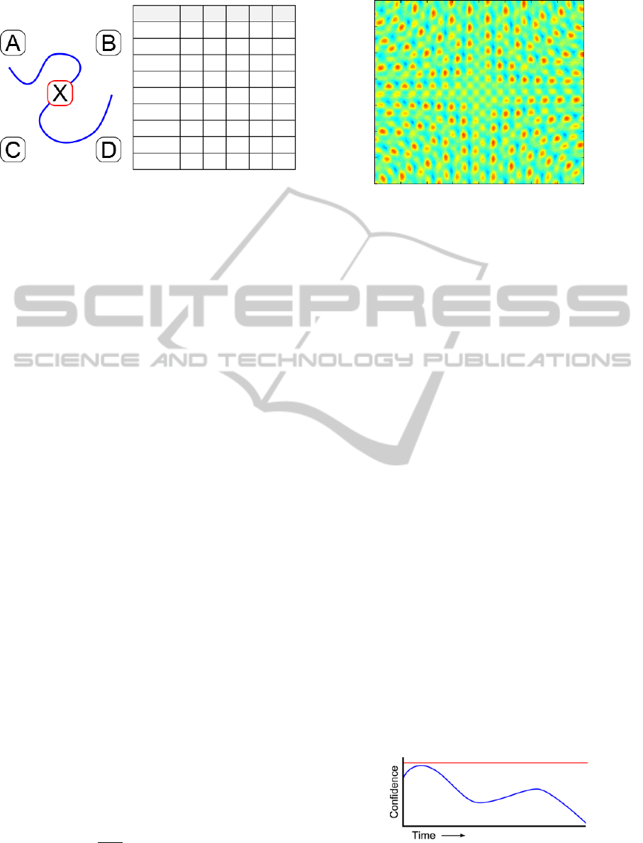
Figure 2: Possible configurations for an infrastructure,
with four infrastructure nodes (A, B, C, D) and one
tracked node (X).
Figure 2. The schedule contains 12 different
configurations, each with 2 transmitters and 2
receivers. Note the moving node is always a receiver
in each configuration, while the other roles are
changing, as shown in Figure 2. Note that
configurations C1-6 and C7-12 are identical except
for the fixed reference receiver, which causes only a
constant bias between the two measured phase
differences in (1).
Note that the number of configurations and the
required time for a measurement round remain
constant with the increasing number of tracked
nodes because the tracked nodes are receivers only.
With more configurations the tracking robustness
and accuracy can be increased.
Note that the experimental results in (Maroti,
2005) show that for radio interferometric
localization or tracking the maximum distance
between the transmitter and the receiver can be
larger than the range of the digital communication.
In our experimental tests the devices used for quad-
range measurement must be in the range of the
digital communication due to the utilized time
synchronization, resulting a range of a few dozens of
meters.
2.3 Interferometric Tracking
In (Zachár, 2014) a novel method was proposed
where the positioning and tracking is performed in a
different way; instead of directly calculating the
position estimator (e.g. as in (Maroti, 2005)) an
intermediate confidence map
,
1
,
is computed for the entire measurement area, with
the following error function:
,
1
∆
,
(2)
Figure 3: Confidence map, measured and calculated by a
measurement setup similar to one in Figure 2.
where p is the position under calculation and k is the
measurement round, producing C measurements for
each c configuration, as follows:
,
,…,
(3)
and ∆ϑ
represents the difference between the ideal
and the measured phase difference values:
∆
,
min
,,
2
(4)
The resulting 2D confidence map shown in Figure 3.
contains several peaks which represent the possible
positions of the object. This provides a possibility to
locate and track all of the possible locations
simultaneously with low computation cost thus
make the tracking feasible in real time.
The map in Figure 3 contains a peak,
corresponding to the true position of the tracked
device, and phantom positions. As the object moves,
the peaks are also moving in the confidence map.
Once the initial position of the object is known, the
tracking problem can trivially be translated into the
problem of following the position of the peak,
corresponding to the true location, in the confidence
map. The method proposed in (Zachár, 2014),
however, goes further and determines the track of a
moving object, even if the initial position is not
known.
The method in (Zachár, 2014) is based upon the
behavior of the peaks in the confidence map: the
confidence value of the peak, which belongs to the
Figure 4: Illustration of the ideal confidence values
corresponding to the true trajectory (red) and a phantom
trajectory (blue).
Config A B C D X
C1 T T R R
C2 T R T R
C3 T R T R
C4 R T T R
C5 R T T R
C6 R T T R
C7 T T R R
…
C12 R T T R
Prediction-aidedRadio-interferometricObjectTracking
163

true position remains constantly high (illustrated by
a red curve in Figure 4), but the confidence values
belonging to phantom positions fluctuate heavily
and eventually disappear (blue curve in Figure 4), as
the object is moving. This feature of the confidence
map makes it possible to distinguish between the
phantom tracks and the real track of the object over
time. The proposed algorithm in (Zachár, 2014)
tracks all of the possible positions as long as the
corresponding peaks in the confidence map are high,
and disposes those phantom tracks, where the peak
value decreases below a limit, thus after a
sufficiently long track only the true trajectory
remains.
Unfortunately the algorithm of (Zachár, 2014)
lacks the possibility to continue a track if a peak is
disappearing for a few measurement rounds due to
e.g. erroneous or missing phase measurements or
faulty peak detection on the confidence map. In
practical situations bad measurements are present,
measurement results may be lost due to
communication problems, and in such cases the
track may be lost. In this paper two means are
proposed to avoid such problems, thus to provide
more robust trajectory estimates.
3 PROPOSED SOLUTION
The proposed solution provides an enhanced and
more robust tracking method based on a confidence
map. The proposed techniques are illustrated in
Figure 5. The original method of (Zachár, 2014)
uses a fixed threshold. As opposed to the ideal case,
illustrated in Figure 4, real measurements often
results in true peaks with smaller amplitude, thus the
original method may lose tracks, as illustrated in
Figure 5(a). The proposed adaptive peak search
method, illustrated in Figure 5(b) and discussed in
Section 3.1, uses an adaptive threshold, thus the
number of peak losses can be decreased (but not
necessarily fully prevented). The peaks, which are
lost for a short time, would result in complete track
loss, which is prevented by the proposed prediction
method, described in Section 3.2: if a track seems to
end, due to the lost peak, the track it is maintained
for a while, using predicted peaks from
neighborhood information. Thus temporary peak
losses can be tolerated, as illustrated in Figure 5(c).
The new tracking algorithm, using adaptive
threshold and predictive track enhancement is
formalized in Section 3.3.
Figure 5: Left column: confidence values of real objects
(red), phantom objects (blue) and the thresholds (green);
Right column: estimated object trajectories. (a) constant
threshold, with two peak-losses, resulting in a track loss,
(b) adaptive threshold, still peak loss possible, causing
track loss, (c) adaptive threshold with prediction, which
tolerates temporary peak losses.
3.1 Adaptive Peak Extraction
The proposed object tracking algorithm operates on
the possible positions, extracted from the peaks of
the confidence map in each measurement round,
thus the quality of the peak extraction heavily
influences the accuracy and robustness of the
tracking. In the case of noisy measurements the
confidence map can be blurred and may contain
multiple smaller peaks rather than one, sharp peak in
a possible position. The proposed solution uses
binarization with an adaptive threshold.
The proposed peak extraction is illustrated in
Figure 6. The algorithm uses the confidence map, as
input (see Figure 6(a)). In the first step high peaks
are selected using the threshold, resulting a new
binary map where peaks higher than the threshold
are represented as blobs, as shown in Figure 6(b). In
the second step, shown in Figure 6(c), possible
positions are determined as the geometric centers of
each region, thus eliminating the issues with blurred
or multiple peaks.
Figure 6: Peak extraction. (a) Confidence map, (b) binary
map, (c) peak position estimation.
SENSORNETS2015-4thInternationalConferenceonSensorNetworks
164
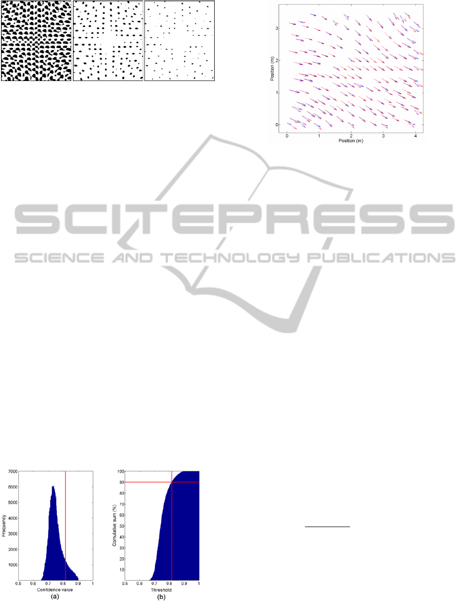
Figure 7: Peak selection with too low (a), correct (b), and
too high (c) threshold.
The key part of the extraction method is the
threshold level selection. An illustrative example is
shown in Figure 7, with peaks selected with too low,
correct, and too high thresholds. In the case of low
threshold value the separate regions are merging (see
Figure 7(a))), while the too high threshold value
causes lower number of detected peaks (see Figure
7(b)). In real cases the confidence values highly
depend on the measurement noise and vary in each
measurement round. Thus a constant threshold
values, as in Figure 5(a), should be avoided.
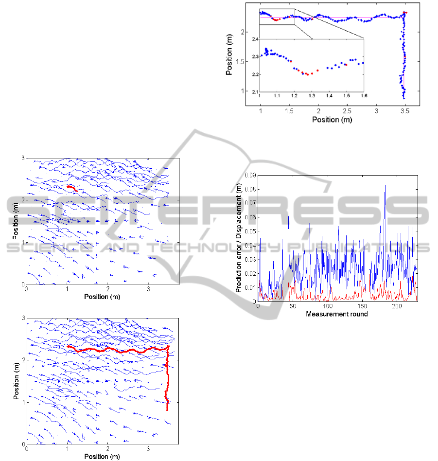
The proposed dynamic threshold value selection
(shown on Figure 5(b)) is based on the histogram of
the confidence map. A typical histogram and
cumulative histogram can be seen in Figure 8(a) and
Figure 8(b), respectively. The dynamic threshold
value is determined as the value where 90% of the
confidence map values are lower than the selected
value, as shown in Figure 8.
3.2 Confidence Map-based Peak
Prediction
The proposed peak prediction method enhances the
tracking robustness by predicting the peaks’
movements based on the confidence map itself.
There are time instances where the confidence value
of a possible position can go below the threshold
value as can be seen on Figure 5(b), which makes
Figure 8: Typical (a) histogram and (b) cumulative
histogram of a confidence map. Red lines show the
selected threshold value.
Figure 9: Illustration of the predictive peak tracking. Blue
arrows show the calculated (true) movement vectors of the
peaks in one iteration, red arrows show the predictions for
the same vectors. For better visibility the vectors were
enlarged.
the associated track impossible to follow. The
original algorithm presented in (Zachár, 2014) marks
the track as dead and stops tracking the real or
phantom object positions in these cases.
In the proposed solution uses three track
attributes: alive, alive but invalid, and dead. Alive
tracks become invalid, when the peak is lost, but
kept alive for a limited number of measurement
rounds. For invalid tracks the position is estimated
from the last known or estimated position (i.e. peak
location).
The proposed solution focuses on solving the
recovery problem; making the tracks alive for a
longer period and assign them to the appropriate
possible position. The key idea can be seen in Figure
9; possible positions of a peak can be estimated in
consecutive measurement rounds using the
confidence map. The displacement of a lost peak can
estimated from the displacement of other peaks in
the close vicinity. This idea is illustrated and also
justified the by Figure 9, where the movement
vectors, calculated from a real measurement, are
approximately the same in a small neighborhood.
Thus the proposed solution predicts the
displacement of a given point P as follows:
∑
,
(5)
where
and
are the initial and the end points of
a nearby movement vector, calculated from two
consecutive confidence maps, and n is the number of
vectors within a specified distance L.
3.3 Tracking Algorithm
The pseudo-code of the tracking algorithm is shown
Prediction-aidedRadio-interferometricObjectTracking
165

Figure 10: Pseudo code of the prediction-aided tracking algorithm.
in Figure 10. The input of the proposed tracking
algorithm in each time instant ( 1,2,…,) is
the measured phase vector
. The vector
length varies depending on the on the number of the
utilized configurations (see Figure 2). The outputs of
the algorithm are the lists of active, inactive and
dead tracks; aTrack, iTrack, dTrack respectively
(see lines 1-2). Ideally the active tracks list contains
only one element which belongs to the real object
movement. At the beginning of the algorithm new
tracks are created for each of the possible positions,
containing the real object position and several
phantom positions (lines 4-13). In each of the
following measurements rounds the new possible
positions are calculated and the movements of the
tracks are computed (lines 14-54). First the new
confidence map is calculated and the peak positions
are identified (lines 15-18). Then each active track is
checked whether a detected peak can be regarded as
the follow-up of the track (line 23). If a track can be
followed then it will be marked as active and the
measured new position is used as the last position of
the track (lines 24-28). If a track cannot be followed
(due to a lost peak) then the new position will be
predicted and the track will be marked as inactive
(lines 30-33). Inactive tracks are similarly handled in
lines 37-50. At the end of the iteration the dead
tracks are separated from the inactive tracks (lines
51-53). The current solution marks a track dead if it
is inactive for
consecutive iterations.
4 EVALUATION
The performance of the proposed algorithm was
tested with real measurements. In the test four
infrastructure nodes and one tracked node were
used. The algorithm utilized all the twelve possible
configurations C1-12 (see Figure 2). The test was
performed in a 4.5 m by 4.5 m room where the
infrastructure nodes were placed in the corners of a
3 m by 3.5 m rectangle, 2 m above the ground level
(at coordinates (0, 0, 2), (0, 3, 2), (3.5, 0, 2), and
(3.5, 3, 2) in Figure 11). The moving node was
1 input: phases(k), k=1..n
2 output: aTrack, iTrack, dTrack
3 function TrackPositions
4 aTrack = {}
5 fTrack = {}
6 dTrack = {}
7 map = genConfidenceMap(phases(1))
8 points = possiblePositions(map)
9 for each p points
10 t= new Track
11 t.add(p)
12 aTrack = aTrack t
13 endfor
14 for each ph phases(2..n)
15 prevPoints = points
16 map = genConfidenceMap(ph)
17 points = possiblePositions(map)
18 ap1 = assignPoints(prev_points,
points, ACTIVE_LEVELS)
19 usedPoints = {};
20 newATrack = {};
21 newITrack = {};
22 for each t aTrack
23 if isAssigned(ap1, t.last)
24 p = getNewPoint(ap1, t.last)
25 t.add(p)
26 t.invalid = 0
27 usedPoints = usedPoints p
28 newAtrack = newAtrack t
29 else
30 p = predict(ap1, t.last)
31 t.add(p)
32 t.invalid = 1
33 newITrack = newITrack t
34 endif
35 endfor
36 iTPos = collectPoints(iTrack)
37 ap2 = assignPoints(iTPos,
points\usedPoints, PREDICT_LEVELS)
38 for each t iTrack
39 if isAssigned(ap2, t.last)
40 p = getNewPoint(ap2, t.last)
41 t.add(p)
42 t.invalid = 0
43 newATrack = newATrack t
44 else
45 p = predict(ap1, t.last)
46 t.add(p)
47 t.invalid = t.invalid + 1
48 newITrack = newITrack t
49 endif
50 endfor
51 dTrack = selectDead(newITrack,Ndead)
52 iTrack = newITrack \ dTrack
53 aTrack = newATrack
54 endfor
SENSORNETS2015-4thInternationalConferenceonSensorNetworks
166
carried in hand by a person (probably causing small
deviations in the range of a few dozens of
millimeters). The tracking results of the proposed
algorithm can be seen in Figure 11, where phantom
and real tracks are shown in blue and red,
respectively. With no prediction (Figure 11(a)) the
tracking failed after a few seconds because of noisy
measurements. With the same measurement data the
proposed algorithm performed well and was able to
follow the movement, since the missing estimates
were successfully replaced by predictions (see
Figure 11(b)). In the test the parameter
was
set to five.
(a)
(b)
Figure 11: Tracking results of the measurement (a)
without and (b) with peak prediction.
Figure 12 shows the reference trajectory in magenta
and the estimated true trajectory. The maximum
deviation from the reference track is 91 mm, part of
which is probably caused by the carrying person.
The estimated and predicted values in Figure 12
are shown in blue and red, respectively. It is
interesting to note that at the magnified part of the
track the predictions follow very well the true
estimated trajectory, despite of the fact that the
Figure 12: The longest track of the measurement. The
estimated and predicted positions are shown with blue and
red dots, respectively. The true track is shown in magenta.
Figure 13: Prediction error (red values) and the lengths of
displacement vectors (blue values) of the real object track.
trajectory changed its direction while only the
predicted values were available. Such prediction,
based on models on the movement itself, would be
very troublesome, but the proposed prediction
scheme using the peaks in the neighborhood handles
the situation properly.
The behavior of the tracking system is illustrated
in Figure 13, where the distances between the
consecutive position estimates are plotted in blue
(missing estimates, shown in red in Figure 12 are
omitted here). The average displacement is 0.023 m,
corresponding to an object speed of approximately
0.25 m/s. The quality of the proposed prediction
scheme is also evaluated in Figure 13. The true track
of the previous measurement (plotted in blue in
Figure 12) was used as reference, and in each
iteration the predicted positions were also calculated
and compared to the estimated positions. The
difference is shown in red in Figure 13. The average
prediction error is 5 mm, while the maximum error
was 21 mm. Clearly the proposed prediction scheme
is able to accurately replace the estimates when they
are not available.
Prediction-aidedRadio-interferometricObjectTracking
167

The experimental results show that the proposed
method is capable of tracking a moving object
equipped with a sensor node device. In contrast to
RIPS (Maroti, 2005) or SRIPS (Dil, 2011), the
proposed tracking algorithm utilizes only one
measurement frequency, resulting shorter
measurement times for each measurement round.
Thus the phase difference measurement errors,
caused by the object movement, can be minimized
and the proposed method is able to provide a robust
tracking, while preserving the few centimeters of
accuracy of the interferometric-based localization
techniques.
5 CONCLUSIONS
In this paper a novel object tracking method was
proposed, which utilizes radio-interferometric phase
measurements and confidence maps. The presented
solution enhances the robustness and quality of the
position estimations when bad measurements are
present or measurements are temporarily missing,
using (1) a new peak detection method utilizing a
dynamic threshold, and (2) by a novel prediction
method, which is able to substitute missing estimates
with predicted positions. The proposed prediction
method examines the evolution of the confidence
map in time and calculates the predicted position
from it, without any external model on the
movement of the tracked object.
The complexity of the proposed algorithm is
moderate thus it can be implemented in real time
using ordinary computers.
The performance of the proposed algorithm was
illustrated and evaluated by real measurements. The
proposed prediction method was validated: the mean
prediction error was typically 5 mm, while the
maximum error was 21 mm during the experiment.
The increased robustness of the algorithm was
clearly shown in the experiments where the
proposed algorithm was able to follow the object
movement with maximum error of 91 mm, despite
of the measurement noise and errors.
ACKNOWLEDGEMENTS
This work was partially supported by the Hungarian
State and the European Union under project
TAMOP-4.2.2.-C-11/1/KONV- 2012-0004.
REFERENCES
Au, A.W.S., et al, 2012. Indoor Tracking and Navigation
Using Received Signal Strength and Compressive
Sensing on a Mobile Device. IEEE Transactions on
Mobile Computing, Vol. 12, No. 10, pp. 2050–2062.
Dil B.J., Havinga, P.J.M., 2011. Stochastic Radio
Interferometric Positioning in the 2.4 GHz Range.
Proceedings of the 9th ACM Conference on Embedded
Networked Sensor Systems (SenSys 11), Seattle, WA,
pp. 108-120.
Kai Ni, Kannan, A., Criminisi, A., Winn, J., 2009.
Epitomic Location Recognition. IEEE Transactions on
Pattern Analysis and Machine Intelligence, Vol.31,
No.12, pp. 2158-2167.
Lanzisera, S., Zats, D., Pister, K. S. J., 2011. Radio
Frequency Time-of-Flight Distance Measurement for
Low-Cost Wireless Sensor Localization. IEEE Sensors
Journal, Vol. 11, No. 3, pp.837-845.
Maroti M., et al, 2005. Radio Interferometric Geolocation.
In ACM Third International Conference on Embedded
Networked Sensor Systems (SenSys 05), San Diego,
CA, pp. 1-12.
Mulloni, A., Wagner, D., Barakonyi, I., Schmalstieg,D.,
2009. Indoor Positioning and Navigation with Camera
Phones, IEEE Pervasive Computing, Vol. 8, No. 2, pp.
22-31.
Peng, C., Shen, G., Zhang, Y., Li, Y., Tan, K., 2007.
BeepBeep: a high accuracy acoustic ranging system
using COTS mobile devices. In Proceedings of the 5th
international conference on Embedded networked
sensor systems pp. 1-14.
Se, S., Lowe, D., Little, J., 2001. Vision-based mobile
robot localization and mapping using scale-invariant
features. Proceedings of 2001 IEEE International
Conference on Robotics and Automation, Vol.2, pp.
2051-2058.
Zachár, G., Simon, G., 2014. Radio-Interferometric Object
Trajectory Estimation. Proc. 3rd International
Conference on Sensor Networks, SENSORNETS 2014,
pp. 268-273.
SENSORNETS2015-4thInternationalConferenceonSensorNetworks
168
