
Adaptive Segmentation based on a Learned Quality Metric
Iuri Frosio
1
and Ed R. Ratner
2
1
Senior Research Scientist, NVIDIA, 2701 San Tomas Expressway, Santa Clara, CA 95050, U.S.A.
2
CTO, Lyrical Labs, 332 South Linn St. Suite 32, Iowa City, IA 52240, U.S.A.
Keywords: Superpixel, Adaptive Segmentation, Machine Learning, Segmentation Quality Metric.
Abstract: We introduce here a model for the evaluation of the segmentation quality of a color image. The model
parameters were learned from a set of examples. To this aim, we first segmented a set of images using a
traditional graph-cut algorithm, for different values of the scale parameter. A human observer classified
these images into three classes: under-, well- and over-segmented. This classification was employed to learn
the parameters of the segmentation quality model. This was used to automatically optimize the scale
parameter of the graph-cut segmentation algorithm, even at a local scale. Experimental results show an
improved segmentation quality for the adaptive algorithm based on our segmentation quality model, which
can be easily applied to a wide class of segmentation algorithms.
1 INTRODUCTION
Segmentation represents a key processing step in
many applications, ranging from medical imaging
(Sun, 2013; Frosio, 2006; Achanta, 2012) to
machine vision (Sungwoong, 2013; Alpert, 2012)
and video compression (Bosch, 2011). Segmentation
algorithms aggregate sets of perceptually similar
pixels in an image (Achanta, 2012; Kaufhold, 2004).
These sets capture image redundancy, they are used
to compute image characteristics and simplify
subsequent image processing.
In the recent past, graph-cut segmentation
algorithms attracted lot of attention because of their
computational efficiency and capability to adhere to
the image boundaries (Achanta, 2012). Most of these
are based on the seminal paper by Felzenszwalb and
Huttenlocher, (Felzenszwalb, 2004), that assert that
a segmentation algorithm should “capture
perceptually important groupings or regions, which
often reflect global aspects of the image.” The
graph-cut algorithm:
(i) builds an undirected graph G = (V, E), where
v
i
∈
V is the set of pixels of the image that has to be
segmented and (v
i
, v
j
)
∈
E is the set of edges that
connects pairs of neighboring pixels;
(ii) associates a non-negative weight w(v
i
, v
j
) to
each edge with a magnitude proportional to the
difference between v
i
and v
j
;
(iii) performs image segmentation by finding a
partition of V such that each component is
connected, the internal difference between the
elements of each component is minimal and the
difference between elements of different
components is maximal.
Figure 1: Panel (a) shows a 640x480 image; panels (b-d)
show the segmentation obtained with the algorithm in
(Felzenszwalb, 2004), with
σ
= 0.5, min size = 5 and k = 3,
100 and 10,000 respectively.
A predicate determines if there is a boundary
between two adjacent components C
1
and C
2
, that is:
()
() ()
>
=
otherwisefalse
CCMIntCCDififtrue
CCD
2121
21
,,
,
, (1)
where Dif(C
1
, C
2
) is the difference between the two
components, defined as the minimum weight of the
283
Frosio I. and Ratner E..
Adaptive Segmentation based on a Learned Quality Metric.
DOI: 10.5220/0005257202830292
In Proceedings of the 10th International Conference on Computer Vision Theory and Applications (VISAPP-2015), pages 283-292
ISBN: 978-989-758-089-5
Copyright
c
2015 SCITEPRESS (Science and Technology Publications, Lda.)

set of edges that connects C
1
and C
2
; Mint(C
1
, C
2
) is
the minimum internal difference, defined as:
( ) () () () ()
[]
221121
,min, CCIntCCIntCCMInt
ττ
++=
, (2)
where Int(C) is the largest weight in the minimum
spanning tree of the component C (and it describes
therefore the internal difference between the
elements of C) and
τ
(C) = k/|C| is a threshold used
to establish whether there is evidence for a boundary
between two components (it forces two small
segments not to fuse if there is strong evidence of
difference between them).
In practice, k is the most significant parameter of
the algorithm, as it sets the scale of observation
(Felzenszwalb, 2004). The authors demonstrated that
the algorithm generates a segmentation that is
neither too fine nor too coarse, but the definition of
fineness and coarseness essentially depends on k that
has to be carefully set to obtain a perceptually
reasonable result. Small k values lead to over-
segmentation (Fig. 1b), whereas a large k may
introduce under-segmentation (Fig. 1d). It is worth
noticing that the definition of a scale parameter is
common in many other superpixel algorithms like
SLIC (Achanta, 2012), where this parameter is
generally referred to as the size of the superpixel.
Assuming that an optimal segmentation algorithm
should extract “perceptually important groupings or
regions”, finding the optimal k for the graph-cut
algorithm (Felzenszwalb, 2004) remains up to now
an open issue. An analogue problem is the selection
of the threshold value used to identify the edges in
edge-based segmentation (Canny, 1986;
Senthilkumaran, 2009). Furthermore, even recently
proposed, efficient superpixel algorithms like SLIC
require a-prori definition of the typical scale of the
segments.
As an attempt to overcome this limitation, we
developed a heuristic model that quantifies the
segmentation quality for a color image. The
parameters of the model were learned from a set of
examples, classified by a human observer into three
classes: under-, well- and over-segmented. We
employed this model to automatically and adaptively
modulate k in graph-cut segmentation, such that a
human observer ideally classifies each part of the
image as well-segmented. We compared then the
segmentation obtained with the proposed method
with the original graph-cut algorithm and with the
recently proposed SLIC, showing that our model
furnishes a reasonable heuristic which can be used to
effectively improve and automate existing
segmentation algorithms.
2 METHOD
2.1 Preliminaries
Fig. 2 shows the block of 160x120 pixels
highlighted in Fig. 1a and segmented with graph-cut
for different values of k. For 1 ≤ k ≤ 50, over-
segmentation occurs: areas that are perceptually
homogeneous are divided into several segments. The
segmentation looks fine for 75 ≤ k ≤ 200, whereas
for 350 ≤ k ≤ 10,000 only few segments are present
(under-segmentation). To derive our segmentation
quality model we need to turn such qualitative
evaluations into a measurable, quantitative index.
To this end, we consider the information in the
original image, img, that is captured by the
segmentation process. We define the color image,
seg, obtained by assigning to each pixel the average
RGB value of the corresponding segment. For each
color channel, {R, G, B}, we compute the symmetric
uncertainty U of img and seg as (Witten, 2002):
{}
{} {}
()
{}{}
seg
BGR
img
BGR
BGRBGR
BGR
SS
segimgI
U
,,,,
,,,,
,,
,2
+
=
, (3)
where S
i
j
indicates the Shannon’s entropy (Witten,
2002), in bits, of the channel i of the image j,
whereas I(u,v) is the mutual information, in bits, of
the images u and v. The symmetric uncertainty
expresses the percentage of bits shared by img and
seg for each color channel; it is zero when the
segmentation is uncorrelated with the original color
image channel, whereas it is one when the
segmentation represents any fine detail (including
noise) in the corresponding channel of img. Since
Figure 2: Weighted uncertainty, U
w
, as a function of k, for
the 160x120 block highlighted in Fig. 1a, segmented with
the graph-cut algorithm in (Felzenszwalb, 2004), for
σ
=
0.5, min size = 5 and k ranging from 1 to 10,000. The
classification into under-, well- or over-segmented class
operated by a human observe is also reported.
VISAPP2015-InternationalConferenceonComputerVisionTheoryandApplications
284

different images have different information in each
color channel (for instance, the image in Fig. 1 has
lot of information in the green channel), we define
the following weighted uncertainty index:
seg
B
seg
G
seg
R
seg
BB
seg
GG
seg
RR
w
SSS
SUSUSU
U
++
⋅+⋅+⋅
=
. (4)
The index U
W
is in the interval [0, 1], and it is
represented in Fig. 2 as a function of k, for the
160x120 block in Fig. 1a. This curve empirically
demonstrates the strict relation between the
segmentation quality and U
W
, which we observed on
a large number of images: U
W
decreases
(approximately monotonically) for increasing k,
passing from over-segmentation to well- and under-
segmentation.
2.2 Segmentation Quality Model
The curve depicted in Fig. 2 represents the specific
case of the 160x120 block in Fig. 1a: U
W
values
Figure 3: Classification of segmented 160x120 sub-images
in the available dataset, performed by a human observer,
represented in the (log(k), U
W
) plane, for image resolutions
of 320x240 (panel (a)) and 640x480 (panel (b)) pixels.
The magenta and red lines represent the boundaries of the
area including the well-segmented sub-images (see text for
details); the green line is the ideal line for segmentation.
associated to a reasonable segmentation in this
specific case may not be adequate for other images.
An image with a lot of small details requires for
instance high U
W
values to represent them all. On the
other hand, small U
W
values are associated to a
reasonable segmentation quality in homogenous
areas, where most of the image information comes
from the image noise and not from image details that
are perceptually important.
To derive a general segmentation quality model,
we have therefore considered a set of 12 images
including flowers, portraits, landscapes and sport
images at 320x240 and 640x480 resolutions. We
divided each image into sub-images of 160x120
pixels and segmented each sub-image with the
graph-cut algorithm in (Felzenszwalb, 2004), for
σ
=
0.5, min size = 5 and k ranging from 1 to 10,000.
Each segmented sub-image was classified by a
human observer as over-, well- or under-segmented
and for each of them we computed U
W
as in Eq. (4).
Fig. 3 shows the results of this classification
procedure. A single value of k cannot be used to
identify well- segmented blocks at a given
resolution, but an area in the (log(k), U
W
) can be
defined for this purpose (notice we used log(k)
instead of k to better highlight the difference along
the horizontal direction). We have therefore divided
the (log(k), U
W
) space into three different regions
representing under-, well- or over-segmented
images, by means of a classifier partially inspired to
Support Vector Machines (Shawe-Taylor, 2004). In
particular, let us consider two classes of points in the
(log(k), U
W
) space, for instance the under- and well-
segmented cases. To estimate the (m, b) parameters
of the curve U
W
= m·log(k) + b that divides these
two regions, we minimized the following cost
function (through the Nelder-Mead simplex):
()
()
()
=
=
⋅
+
+−⋅
+⋅
+
+−⋅
=
WE
US
N
i
iWE
iWi
N
i
iUS
iWi
m
bUkm
m
bUkm
bmE
1
,
2
,
1
,
2
,
1
log
1
log
,
δ
δ
, (5)
where N
US
and N
WE
are respectively the number of
under- and well-segmented points and
δ
US,i
and
δ
WE,i
are 0 if the point is correctly classified (i.e., for any
under-segmentation point that does not lie under the
U
W
= m·log(k) + b curve) and 1 otherwise. The cost
function in Eq. (5) is the sum of the distances from
the line U
W
= m·log(k) + b of all the points that are
misclassified. The estimate of the two lines that
divide the (log(k), U
W
) is performed independently.
Finally, the average line between these two (in green
in Fig. 3) is assumed to be the optimal line for
AdaptiveSegmentationbasedonaLearnedQualityMetric
285
segmentation in the (log(k), U
W
) plane.
In the next section, we will detail how this learned
model can be used to automatically identify the
optimal k and to subsequently develop a spatially
adaptive segmentation algorithm. With this aim, it is
important to remember that we have experimentally
observed an approximately monotonic, S-shaped
curve U
W
= U
W
[log(k)] in the (log(k), U
W
) space for
each sub-image (Figs. 2 and 3): for small k values,
U
W
is constant and over-segmentation occurs;
increasing k, U
W
decreases rapidly and well-
segmented data are observed in this area; finally, for
large k, under-segmentation occurs and a new
plateau is observed on the curve. Given the shape of
the typical U
W
= U
W
[log(k)] curve in the (log(k),
U
W
), a point of intersection between the optimal line
for segmentation and the U
W
= U
W
[log(k)] curve can
always be identified. This observation represents the
key idea for the development of the estimate of the
optimal k parameter described in the next Section.
3 RESULTS
3.1 Automatic Identification of K
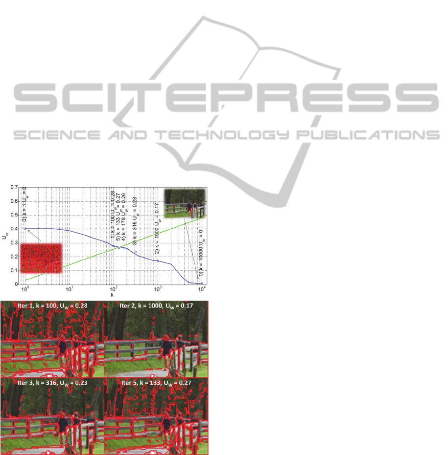
Figure 4: Iterative estimate of k for a 160x120 sub-image.
The iterative process is shown in the (log(k), U
W
) plane in
the upper panel. The lower panels show the corresponding
segmentations. Convergence is reached after 5 iterations.
The optimal line for segmentation, m·log(k) + b,
constitutes a set of points in the (log(k), U
W
) that are
associated to well-segmented sub-images by a
human observer. Given a 160x120 sub-image, the
optimal k is defined here as the one that generates a
segmentation whose weighted symmetric
uncertainty U
W
is as close as possible to m·log(k)+ b.
Such value is computed iteratively through a
bisection approach: at iteration 0, the sub-image is
segmented for k
Left
= 1 and k
Right
= 10,000 and the
corresponding values of U
W,Left
and U
W,Right
are
computed. At the next iteration, the mean log value
(k = exp{[log(k
Left
)+log(k
Right
)]/2}) is used to
segment the sub-image, the corresponding U
W
is
computed and k
Left
or k
Right
are substituted to k,
depending on the fact that (log(k
Left
), U
W,Left
), (log(k),
U
W
), and (log(k
Right
), U
W,Right
) lie under or above the
optimal segmentation line. Fig. 4 illustrates this
iterative procedure: the initial values of k clearly
lead to strong under- or over-segmentation, but after
5 iterations the image segmentation appears
reasonable and the corresponding point in the
(log(k), U
W
) space lies close to the optimal
segmentation line.
3.2 Adaptive Selection of K
To segment a 320x240 or 640x480, a set of adjacent
sub-images has to be considered. Nevertheless,
putting together the independent segmentations of
each sub-image does not produce a satisfying
segmentation, since segments across the borders of
the sub-images are divided into multiple segments.
We have therefore modified the original graph-cut
segmentation algorithm in (Felzenszwalb, 2004) to
obtain an iterative algorithm that makes use of an
adaptive scale factor k(x, y), instead of the constant
parameter used in the original algorithm (the
threshold function in Eq. (2), thus becomes
τ
(C, x, y)
= k(x, y)/|C|).
The scale map k(x, y) was obtained with the
following procedure; first, the image was segmented
using k(x, y) =1 and k(x, y) =10,000 for all the image
pixels. Then, for each 160x120 sub-image and
independently from the other sub-images, the value
of k was updated through the iterative procedure
detailed in Section 3.1 and assigned to all the pixels
of the sub image; the adaptive scale factor k(x, y)
was finally smoothed through a low pass filter to
avoid sharp transition of k(x, y) along the image.
3.3 Results on Real Images
For the proposed adaptive graph-cut algorithm, the
VISAPP2015-InternationalConferenceonComputerVisionTheoryandApplications
286
original graph-cut in (Felzenszwalb, 2004) (using
σ
= 0.5, min size = 5 in both cases)
and SLIC
(Achanta, 2012), we computed three indexes to
quantify the quality of the segmentation algorithms
on a set of 36 images at 320x240 and 640x480. It is
worthy to notice that the authors of SLIC consider
the graph-cut segmentation algorithm by
Felzenszwalb and Huttenlocher one of the first
superpixel algorithm, thus making this comparison
particularly significant.
Notice that multiple indexes are necessary to
evaluate the quality of segmentation, because of the
different aspects to be considered at the same time
(Chabrier, 2004; Gelasca, 2004; Beghdad, 2007).
The three indexes considered here are the Inter-class
contrast, Intra-class uniformity (Chabrier, 2004), and
their ratio. The first index measures the average
contrast between the different segments, and it is
generally higher for high quality segmentation
(although the contrast between different segments
can be lower if the segmentation contains textures).
The Intra-class uniformity measures the sum of the
normalized standard deviations of the segments and
it should be low for high quality segmentation
(although it also increases when the image contains
a lot of texture and/or noise). We also used the ratio
between these two indexes to obtain a first,
normalized index that depends less on the presence
of texture and noise.
During the testing, we first segmented the images
using the proposed, adaptive graph-cut algorithm,
which does not require any additional input
parameter. For the original graph-cut algorithm, we
set k to obtain the same number of segments
obtained with the proposed adaptive version of the
same algorithm. The number of superpixels in SLIC
was set following the same principle, whereas the
compactness parameter was fixed to 20.
The indexes measured over all the images of our
dataset, together with their average and median
value, are reported in table 1 and 2 for the 320x240
and 640x480 resolutions, respectively. The proposed
method has the higher Inter-class contrast at both
resolutions, thus suggesting that it separates different
object better than the original graph-cut algorithm
and SLIC. When Intra-class uniformity is
considered, SLIC achieves the best result for
320x240 resolution, but at 640x480 resolution the
proposed adaptive graph-cut algorithm has the
lowest Intra-class uniformity. These results are
overall consistent with the recent literature (Achanta,
2012), reporting that SLIC is characterized by lower
boundary recall with respect to the graph-cut
algorithm: it produces a set of regular, uniform
superpixels, but it also possibly includes in the same
segments areas occupied by different objects in the
image. This issue is however less evident at the low
320x240 resolution, where object boundaries are less
to SLIC further confirm that, when these quality
indexes are considered, the segmentation obtained
with the proposed method is qualitatively superior
with respect to that produced by SLIC.
Table 1: Inter-class contrast, Intra-class uniformity and
their ratio for the graph-cut algorithm in (Felzenszwalb,
2004), its adaptive version developed here and SLIC, for
our testing set of images at 320x240 resolution.
# image
Adaptive Graph-Cut
Graph-Cut
SLIC
Adaptive Graph-Cut
Graph-Cut
SLIC
Adaptive Graph-Cut
Graph-Cut
SLIC
10.410.41 0.33 11.58 12.72 7.45 35.80 32.01 44.81
2 0.16 0.16 0.17 7.25 7.47 7.14 21.45 20.95 24.42
3 0.18 0.18 0.18 5.01 5.42 4.02 35.71 32.74 45.99
4 0.23 0.23 0.21 15.49 15.57 18.02 14.64 14.86 11.45
50.270.25 0.20 17.96 19.84 18.16 15.21 12.68 11.21
6 0.15 0.15 0.14 5.07 5.41 5.53 29.11 27.83 25.13
70.320.29 0.22 6.19 5.98 4.02 51.65 48.18 54.63
80.250.23 0.20 13.56 13.35 18.04 18.66 17.34 11.09
90.150.14 0.11 2.10 2.34 2.32 70.78 59.36 46.76
10 0.11 0.11 0.10 6.52 6.92 5.48 16.19 15.21 18.34
11 0.26 0.26 0.18 23.17 22.52 15.22 11.42 11.73 11.89
12 0.37 0.38 0.27 2.55 2.65 1.90 146.25 143.87 143.39
13 0.04 0.04 0.03 0.15 0.14 0.15 244.01 261.14 162.06
14 0.11 0.10 0.08 6.12 5.84 5.69 17.48 16.84 14.82
15 0.06 0.05 0.05 6.44 6.66 6.67 8.68 8.10 6.83
16 0.20 0.19 0.15 17.33 19.48 10.85 11.33 9.76 14.03
17 0.27 0.26 0.22 13.58 13.89 14.17 19.84 18.83 15.43
18 0.16 0.14 0.12 7.23 7.59 5.41 22.22 18.01 21.28
19 0.09 0.09 0.07 3.45 3.72 0.99 24.88 24.64 66.31
20 0.18 0.12 0.10 15.76 16.89 17.97 11.53 7.09 5.79
21 0.14 0.13 0.10 13.19 13.71 11.34 10.87 9.73 9.04
22 0.07 0.06 0.04 6.88 6.91 6.40 10.48 9.23 6.87
23 0.11 0.10 0.07 9.96 9.70 9.45 11.07 10.26 7.55
24 0.21 0.22 0.18 7.44 7.42 8.63 28.72 29.02 20.41
25 0.17 0.17 0.15 25.09 25.81 26.82 6.97 6.56 5.77
26 0.19 0.18 0.15 16.10 16.36 14.44 11.71 11.27 10.27
27 0.15 0.15 0.11 8.78 9.10 8.50 17.13 16.56 13.25
28 0.14 0.14 0.12 20.27 20.64 17.36 6.90 6.95 7.06
29 0.14 0.13 0.12 2.38 2.42 2.17 58.45 55.37 57.26
30 0.26 0.24 0.24 10.95 10.66 7.91 23.45 22.56 30.43
31 0.20 0.20 0.20 9.40 9.81 10.42 21.62 20.59 18.83
32 0.17 0.17 0.16 17.13 18.59 16.83 9.82 9.04 9.40
33 0.28 0.24 0.20 20.09 21.21 19.03 13.81 11.51 10.32
34 0.24 0.24 0.21 38.56 38.62 39.46 6.28 6.23 5.24
35 0.30 0.25 0.16 12.34 13.64 12.89 24.58 18.42 12.12
36 0.20 0.20 0.15 34.96 36.41 40.91 5.77 5.49 3.73
Average 0.19 0.18 0.15 12.22 12.65 11.72 30.40 29.17 27.31
Median 0.18 0.17 0.15 10.45 10.23 9.04 17.30 16.70 13.64
320x240
Inter-class
contrast
Intra-class
uniformity 1000 * Inter /Intra
AdaptiveSegmentationbasedonaLearnedQualityMetric
287

Table 2: Inter-class contrast, Intra-class uniformity and
their ratio for the graph-cut algorithm in (Felzenszwalb,
2004), its adaptive version developed here and SLIC, for
our testing set of images at 640x480 resolution.
precisely defined because of the low number of
pixels. The average and median value of the of Inter-
class contrast/Intra-class uniformity ratio of the
proposed adaptive graph-cut algorithm with respect
to SLIC further confirm that, when these quality
indexes are considered, the segmentation obtained
with the proposed method is qualitatively superior
with respect to that produced by SLIC.
It can also be noticed that the average and
median quality indexes are better for the adaptive
version of the graph-cut algorithm compared to its
original formulation. The only exception is the
average of Inter-class contrast / Intra-class
uniformity ratio. However, this fact is explained
considering that, for image #13 in our dataset, this
algorithm achieves a very large Inter/Intra ratio. This
is not surprising given that the Intra-class uniformity
measure does a poor job of evaluating segmentation
quality in cases of highly textured segments or
segments with smooth color gradients (like in the
case of image #3, see Fig. 6), though it is a very
useful measure in many other cases. Thus with truly
better segmentation, we would, in general, expect a
smaller Intra-class value, but we would expect
notable exceptions. This is, exactly, what we
observe.
Fig. 5 shows two typical segmentation results
obtained on 640x480 images; the same figure shows
the corresponding scale maps k(x, y) and the
segmentation achieved with the original graph-cut
algorithm (Felzenszwalb, 2004) and with SLIC.
When the segmentation quality model derived in
Section 2 is used to adaptively set k(x, y), large
segments are used in the uniform areas of the image,
like the sky in Fig. 5b as well as the road and the
grass areas in Fig. 5f. These areas are on the other
hand over-segmented when the original graph-cut
algorithm is used. The scale map in Fig. 5a,
associated to the segmented image in Fig. 5b, shows
how the quality segmentation model tends to favor a
large scale in the homogeneous area of the sky and
skyscrapers, thus preventing over-segmentation in
the sky area, which is on the other hand present in
the upper right area of Fig. 5c. The proposed
adaptive segmentation procedure also leads to a finer
segmentation in the upper right area of the second
image in Fig. 5, where many small leaves are present
(Fig. 5f-g).
Fig. 6 shows the segmentation of images #2, #4,
and #13 in the testing set obtained with the different
algorithms considered here. SLIC achieves the best
inter-class contrast and intra-class uniformity for
image #2, since lots of details in the image
background match the scale of the superpixels. This
does not happen for image #4, where the adaptive
algorithm proposed here is capable to adapt the size
of the segments at best (and it also identifies the
boundary between the roof and the sky better than
# image
Adaptive Graph-Cut
Graph-Cut
SLIC
Adaptive Graph-Cut
Graph-Cut
SLIC
Adaptive Graph-Cut
Graph-Cut
SLIC
10.360.36 0.28 22.9 25.6 16.0 15.9 14.0 17.2
2 0.15 0.15 0.15 14.0 14.3 13.3 10.7 10.4 11.6
30.170.16 0.16 11.0 12.2 8.6 15.0 13.3 18.5
40.210.20 0.17 40.7 42.0 43.8 5.1 4.8 3.9
50.220.20 0.17 60.6 68.3 62.7 3.7 2.9 2.7
60.140.13 0.11 7.1 8.0 9.0 19.4 15.7 12.4
70.230.21 0.16 17.9 20.3 9.4 12.8 10.3 17.4
80.230.17 0.16 38.0 42.7 44.3 5.9 4.0 3.6
90.130.12 0.08 5.3 5.8 4.7 24.5 20.2 17.4
10 0.09 0.10 0.09 12.1 13.0 9.6 7.8 7.5 9.1
11 0.19 0.19 0.15 56.0 57.5 40.8 3.5 3.2 3.6
12 0.25 0.31 0.21 5.4 5.7 3.5 45.5 53.8 60.6
13 0.03 0.03 0.02 0.3 0.2 0.3 85.1 142.2 59.3
14 0.09 0.08 0.07 29.7 29.9 30.0 3.2 2.6 2.2
15 0.05 0.05 0.04 21.3 22.6 25.3 2.3 2.1 1.7
16 0.17 0.16 0.13 47.3 58.5 32.3 3.6 2.8 4.1
17 0.24 0.24 0.20 45.1 47.6 48.3 5.3 5.0 4.2
18 0.13
0.11 0.09 23.4 25.1 17.8 5.6 4.4 5.3
19 0.06 0.06 0.05 4.7 9.2 3.1 12.3 6.9 14.5
20 0.15 0.13 0.11 89.2 89.6 128.3 1.7 1.4 0.9
21 0.14 0.12 0.10 65.9 66.6 75.5 2.1 1.9 1.3
22 0.07 0.06 0.05 36.3 36.2 39.1 1.9 1.7 1.3
23 0.10 0.09 0.07 44.8 44.8 52.1 2.2 2.1 1.3
24 0.18 0.17 0.14 18.7 20.4 18.4 9.7 8.5 7.7
25 0.16 0.15 0.13 93.0 95.1 119.8 1.7 1.6 1.1
26 0.16 0.15 0.14 47.0 49.0 49.0 3.5 3.1 2.8
27 0.14 0.12 0.10 31.8 32.9 43.3 4.4 3.5 2.3
28 0.12 0.11 0.11 48.7 51.4 43.9 2.5 2.2 2.5
29 0.13 0.13 0.09 3.3 3.6 3.9 39.2 35.1 24.3
30 0.22 0.22 0.19 18.8 23.1 14.8 11.6 9.5 12.7
31 0.18 0.18 0.16 19.9 21.0 23.8 9.3 8.4 6.5
32 0.14 0.14 0.13 37.9 39.5 37.5 3.8 3.5 3.5
33 0.19 0.18 0.17 44.8 47.5 43.0 4.3 3.7 4.0
34 0.24 0.23 0.21 123.8 129.9 139.5 2.0 1.8 1.5
35 0.18 0.17 0.13 26.6 26.7 33.9 6.9 6.4 3.9
36 0.17 0.17
0.15 69.9 72.5 91.1 2.4 2.4 1.7
Average 0.16 0.15 0.13 35.6 37.7 38.3 11.0 11.8 9.7
Median 0.16 0.15 0.13 30.7 31.4 33.1 5.2 4.2 3.9
640x480
Inter-class
contrast
Intra-class
uniformity
1000 * Inter
/Intra
VISAPP2015-InternationalConferenceonComputerVisionTheoryandApplications
288

Figure 5: Panels (b-d) and (f-h) show images #16 (first row) and #28 (second row) in our 640x480 resolution testing set,
segmented with the adaptive graph-cut algorithm, the original graph-cut algorithm (Felzenszwalb, 2004) and SLIC
(Achanta, 2012). Panels (a) and (e) show the scale maps k(x, y) for the adaptive graph-cut algorithm.
Figure 6: Segmentation of images #2, #4, and #13 in our 640x480 resolution testing set, obtained with different algorithms.
the original graph-cut algorithm) and therefore
achieves the best inter-class contrast and intra-class
uniformity. Finally, graph-cut work at best for these
indexes on the almost homogeneous image #13,
although the superiority of graph the proposed
adaptive graph-cut is questionable at visual
inspection in this case (see for instance how the
proposed approach uses a smaller number of
segments in the sky area and better fits the boundary
of the clouds, Fig. 6g-h).
A final remark is to be made about the
computational costs of the segmentation algorithms
considered here. SLIC is the fastest algorithm, with
a linear complexity with respect to the number N of
AdaptiveSegmentationbasedonaLearnedQualityMetric
289

superpixels, whereas graph-cut has N·logN
complexity. The complexity of the proposed method
is the highest: it is N·logN and it increases linearly
with the number of iterations required to reach the
convergence, which we experimentally observed to
occur typically in less than 7 iterations.
4 DISCUSSION
A wide array of literature on segmentation
algorithms exists based on the main idea expressed
in (Felzenszwalb, 2004) that any segmentation
algorithm should “capture perceptually important
groupings or regions”. Many authors have implicitly
defined the perceptive saliency of an image feature
on the basis of some well-established mathematical
rule: for instance the k parameter in (Felzenszwalb,
2004) defines the typical scale of the image
segments. In SLIC, a similar role is played by the
approximate number of desired segments which is
passed as input parameter, as the superpixels are
spread uniformly across the entire image. A trial-
and-error procedure is however required to set these
parameters such that the segments are perceptually
significant for a human observer. The same issue is
in common with many other segmentation
algorithms, whose output critically depends on the
choice of the input parameters (Sun, 2013;
Sungwoong, 2013; Alpert, 2012; Bosch, 2011).
To overcome this problem, we have developed a
segmentation quality model whose parameters were
learned from a set of segmentation data classified by
a human observer. The resulting segmentation
quality is therefore related to the fact that regions or
objects that are perceptually important for a human
observer are grouped in a same segment. The
segmentation quality model is particularly suited for
applications like medical imaging and video
compression, where the segmented images (or the
compressed video stream) are intended for human
observers.
Based on the proposed segmentation quality
model, we developed a parameter-free algorithm,
which constitutes a significant improvement with
respect to more traditional algorithms requiring
input parameters, whose adequacy has to be verified
a posteriori. The procedure adopted to learn the
model parameters has been applied here specifically
to the graph-based segmentation algorithm in
(Felzenszwalb, 2004). Nevertheless, such procedure
is far more general and ideas detailed in this paper
can be easily applied to other segmentation
algorithms requiring one or more input parameters,
like (Senthilkumaran, 2009; Prakash, 2004). We
have for instance developed and tested a similar
segmentation quality model for edge thresholding
segmentation in the YUV space (Canny, 1986),
achieving similar results (not shown here for reason
of space). We are also going to investigate the
application of the same procedure to develop a
parameter-free version of SLIC (Achanta, 2012) and
to automatically adapt the scale parameter from
region to region within the same image. Notice that,
in this case, two parameters (number of superpixels
and compactness) should be adapted: the optimal
segmentation line becomes in this case a plane (and
more generally, for algorithms with a higher number
of input parameters, an hyper-plane).
It is worthy noticing that the optimal
segmentation line in the (log(k), U
W
) space for the
320x240 resolution (Fig. 3a) is lower than the
optimal line for 640x480 images (Fig. 3b). Thus,
although we considered sub-images of 160x120
pixels for both resolutions, the parameters of the
segmentation quality model change with the image
resolution. This seems reasonable, since at higher
resolution more details are generally visible in the
image, thus requiring a finer segmentation (i.e.,
higher U
w
). The application of the segmentation
quality model to other image resolutions requires
therefore re-classifying segmented sub-images of
160x120 pixels for the given resolution. Another
approach would interpolate the model parameters.
The choice of sub-images of this particular size
was made as a compromise between the need to
include a significant set of image features in the sub-
image (sub-images that are too small could in fact
contain a unique segment and in this case their
classification in under-, well- or over-segmented is
meaningless) and the need to obtain a significantly
high number of sub-images. This last need has two-
fold advantages: first, it is well known that using a
large amount of data significantly improves the
training process in machine learning (Witten, 2002);
this principle is used here to reliably learn the
parameters of the segmentation quality model. As a
second point, optimizing the segmentation
parameters on small 160x120 sub-images allowed us
to develop an adaptive segmentation algorithm by
dividing a full resolution image in a set of sub-
images and computing the optimal scale parameter
for each of them. We were therefore able to develop
an adaptive algorithm, which is intrinsically more
robust and accurate than other procedures using a
single parameter for the entire image (Felzenszwalb,
2004; Isa, 2009).
The results reported in Tables 1 and 2
VISAPP2015-InternationalConferenceonComputerVisionTheoryandApplications
290

demonstrate that the adoption of the proposed
adaptive strategy for the computation of k(x, y) leads
to segments that have more contrast one with respect
to the other and that are more uniform, thus
demonstrating an overall increase in segmentation
quality. Comparison with SLIC shows that
optimizing the segmentation quality using the
proposed model generally leads to a semantic
segmentation, where large objects perceptually
recognized as a single class are effectively described
by a unique segment; this however requires a higher
computational time. On the other hand, SLIC
produces in a short a regular grid of superpixels,
which is more suited for further processing by other
algorithms.
Figs. 5 and 6 show that the proposed method
generally identifies the scale of the objects that are
important for a human observer: for instance
segments are larger close to people in Fig. 5f or in
the homogeneous sky area in Fig. 5b. Nevertheless,
we have also noticed that the proposed algorithm
sometimes produces sets of segments that are too
fine, such as in the left river area in Fig. 5b. Such
sub-optimal behavior has to be investigated more in
detail in the future. To this aim, we are planning to
use the Berkeley segmentation dataset (Martin,
2001) to build a large training set including
hundreds of images semantically segmented by
several human observers, so to significantly improve
the training of the segmentation quality model.
To summarize, the proposed segmentation
quality model can be used to perform segmentation
with no supervision, using an algorithm that
automatically adapts its parameter along the image
to generate a segmentation map that is perceptually
reasonable for a human observer. This is
particularly important in applications like video-
encoding; in this case, it can also be noticed that the
computational cost of the proposed method can be
significantly reduced. In fact, when applied to a
unique frame, the proposed method performs a
search for the optimal k value for each sub-image
considering the entire valid range for k. On the other
hand, since adjacent frames are highly correlated in
video, the range for k can be significantly reduced
considering the estimates obtained at previous
frames for the same sub-image.
REFERENCES
R. Achanta, A. Shaji, K. Smith, A. Lucchi, P. Fua, S.
Süsstrunk, SLIC Superpixels Compared to State-of-
the-art Superpixel Methods, IEEE TPAMI, 2012.
S. Alpert, M. Galun; A. Brandt, R. Basri, Image
Segmentation by Probabilistic Bottom-Up
Aggregation and Cue Integration, IEEE TPAMI, 2012.
A. Beghdad, S. Souidene, An HVS-inspired approach for
image segmentation evaluation, IEEE ISSPA, 2007.
M. Bosch, Z. Fengqing, E. J. Delp, Segmentation-Based
Video Compression Using Texture and Motion
Models, IEEE Journ. Sel. Topics in Sig. Proc., 2011.
J. Canny, A Computational Approach to Edge Detection,
IEEE TPAMI, 1986.
S. Chabrier, B. Emile, H. Laurent, C. Rosenberger, P.
Marché, Unsupervised Evaluation of Image
Segmentation: Application to multi-spectral images,
ICPR, 2004.
P. F. Felzenszwalb, D. P. Huttenlocher, Efficient Graph-
Based Image Segmentation, IJCV, 2004.
E. D. Gelasca, et al., Towards Perceptually Driven
Segmentation Evaluation Metrics, in CVPRW, 2004.
I. Frosio, G. Ferrigno, N. A. Borghese, Enhancing Digital
Cephalic Radiography with Mixture Model and Local
Gamma Correction, IEEE TMI, 2006.
J. Kaufhold, and A. Hoogs, Learning to segment images
using region-based perceptual features, in CVPR,
2004.
N. A. M. Isa, S. A. Salamah, U. K. Ngah, Adaptive fuzzy
AdaptiveSegmentationbasedonaLearnedQualityMetric
291

moving K-means clustering algorithm for image
segmentation, IEEE TCE, 2009.
D. Martin, C. Fowlkes, D. Tal, J. Malik, A Database of
Human Segmented Natural Images and its Application
to Evaluating Segmentation Algorithms and
Measuring Ecological Statistics, ICCV, 2001.
A. Prakash, E. R. Ratner, J. S. Chen, D. L. Cook. Method
and apparatus for digital image segmentation. U.S.
Patent 6,778,698, 2004.
R. Raina, A. Madhavan, A. Y. Ng., Large-scale deep
unsupervised learning using graphics processors,
ICML, 2009.
N. Senthilkumaran, R. Rajesh, Edge detection techniques
for image segmentation–a survey of soft computing
approaches, Int. Journ. Recent Trends in Eng., 2009.
J. Shawe-Taylor, N. Cristianini, Kernel Methods for
Pattern Analysis, 2004.
S. Sun, M. Sonka, R. R. Beichel, Graph-Based IVUS
Segmentation With Efficient Computer-Aided
Refinement, IEEE TMI, 2013.
K. Sungwoong, S. Nowozin, P. Kohli, C. D. Yoo, Task-
Specific Image Partitioning, IEEE TIP, 2013.
I. H. Witten, F. Eibe, Data Mining: Practical Machine
Learning Tools and Techniques, 2002.
VISAPP2015-InternationalConferenceonComputerVisionTheoryandApplications
292
