
LDA Combined Depth Similarity and Gradient Features for Human
Detection using a Time-of-Flight Sensor
Alexandros Gavriilidis, Carsten Stahlschmidt, J
¨
org Velten and Anton Kummert
Faculty of Electrical Engineering and Media Technologies, University of Wuppertal, D-42119 Wuppertal, Germany
Keywords:
Human Detection, Depth Image Features, LDA Feature Combination, Video Processing.
Abstract:
Visual object detection is an important task for many research areas like driver assistance systems (DASs),
industrial automation and various safety applications with human interaction. Since detection of pedestrians is
a growing research area, different kinds of visual methods and sensors have been introduced to overcome this
problem. This paper introduces new relational depth similarity features (RDSF) for the pedestrian detection
using a Time-of-Flight (ToF) camera sensor. The new features are based on mean, variance, skewness and
kurtosis values of local regions inside the depth image generated by the Time-of-Flight sensor. An evaluation
between these new features, already existing relational depth similarity features using depth histograms of
local regions and the well known histogram of oriented gradients (HOGs), which deliver very good results
in the topic of pedestrian detection, will be presented. To incorporate more dimensional feature spaces, an
existing AdaBoost algorithm, which uses linear discriminant analysis (LDA) for feature space reduction and
new combination of already extracted features in the training procedure, will be presented too.
1 INTRODUCTION
Conventional camera systems capturing only avail-
able light of the surrounding area have many bene-
fits as well as drawbacks for the task of visual pedes-
trian detection. Benefits of passive camera systems
are, beside the financial point, the usability for many
different tasks, like pattern recognition, object detec-
tion and image registration. The lighting conditions
are the strongest limitation factors for conventional
camera systems. Relating to pedestrian detection, the
appearance, e.g. color of clothes, and the contrast of
the pedestrian to the background are typical problems
for conventional monocular (Enzweiler and Gavrila,
2009) or stereo (Keller et al., 2011) camera systems.
Besides cues for detection of pedestrians which are
exhaustive evaluated in (Doll
´
ar et al., 2012), informa-
tion about the distance to a detected object are essen-
tial for many assistance systems. The estimation of
a distance to a detected object based on camera cali-
bration and conventional monocular camera systems
is a typical problem too. To overcome such prob-
lems, sensors like Time-of-Flight (ToF) cameras, also
called RGB-D cameras, can be used. In (Ikemura
and Fujiyoshi, 2010) relational depth similarity fea-
tures (RDSFs) for the detection of pedestrians have
been introduced, which are extracted from a depth
image captured by a TOF camera. Based on a max-
imum range resolution of 7.5m of the TOF camera,
a depth image will be quantized into 25 bins, where-
upon each bin has a range resolution of 0.3m. For a
rectangular region, the depth histogram will be cre-
ated using the occurrence of pixel inside each bin of
the 25 quantization steps. After normalization of the
histogram, the Bhattacharyya distance between two
different rectangular regions inside the image will be
calculated and the scalar result will be used as feature
for an AdaBoost classifier. The time of computing
the 25 integral images, as well as the evaluation of the
Bhattacharyya distance over two 25-dimensional his-
tograms for many different rectangular region combi-
nations can be very expensive.
Another approach like (Mattheij et al., 2012) eval-
uates the well known Haar-like features from (Viola
and Jones, 2001b) on depth images and shows that
Haar-like features can deliver accurate results com-
bined with a fast calculation time using integral im-
ages. Histogram of Depth Differences (HDD) de-
veloped in (Wu et al., 2011) and derived from the
Histogram of Oriented Gradients (HOGs) (Dalal and
Triggs, 2005) is nearly the same. The only difference
is the use of the whole 360 degrees of the possible ori-
entations and not just the 180 degrees as described in
(Dalal and Triggs, 2005) of the HOG feature.
349
Gavriilidis A., Stahlschmidt C., Velten J. and Kummert A..
LDA Combined Depth Similarity and Gradient Features for Human Detection using a Time-of-Flight Sensor.
DOI: 10.5220/0005257403490356
In Proceedings of the 10th International Conference on Computer Vision Theory and Applications (VISAPP-2015), pages 349-356
ISBN: 978-989-758-089-5
Copyright
c
2015 SCITEPRESS (Science and Technology Publications, Lda.)

In (Spinello and Arras, 2011) the Histogram of
Oriented Depths (HOD) feature will be introduced,
that has been also derived from the HOG feature. The
HOD will be calculated in the depth image and used
by a soft linear support vector machine (SVM) to de-
tect pedestrians. To improve the decision of the HOD,
a so called Combo-HOD will be introduced that uses
two detectors trained each on either the depth image
with HOD features or the intensity (grayscale) image
with HOG features and combines in that case the sen-
sor cues of each image. The Combo-HOD promises
more accurate precision than the single detectors on
either the depth or the RGB image.
Based on the idea of local binary pattern (LBP),
in (Wang et al., 2012) so called pyramid depth self-
similarities (PDSS) are introduced, which will be
used with a depth image. The core part is to com-
pare local areas in the manner of LBP features, e.g. to
compare a cell (an image area) of a detection window
with its neighbouring cells, by use of histogram inter-
section methods. To concatenate the histograms by a
spatial pyramid over the depth image is a time con-
suming task too. To be as fast and accurate as pos-
sible, the presented approach of this paper is based
on features which are also comparing the relation in
depth of two different areas, but can be computed very
fast, like Haar-like features. Time consuming features
can be used to increase the performance in addition to
the weak features, which will be introduced later in
this paper.
The remainder of the paper is structured as fol-
lows, the next section gives an overview of the used
sensor, the available sensor data and other basic re-
flections regarding the difference between intensity
and depth images. The available features for pedes-
trian detection in 2.5D (RGB-D) data will be de-
scribed in section three. Section four describes the
used classifier and the usage of high dimensional fea-
tures by linear discriminant analysis (LDA) transfor-
mation. The following section show up the results of
the paper and in the last section, a summary and con-
clusions will be given.
2 PRELIMINARY
CONSIDERATIONS
The used ToF camera is the CamCube 3.0 from PMD
Technologies GmbH with a maximum measurement
range of up to 7.5m for the available depth image.
Field of view of the ToF camera is 40 degrees in both
directions with a pixel resolution of (200 × 200) by
a possible frame rate of over 30 frames per second
(fps). A general image can be described by pixel val-
ues g = f (n) with f : n → g, g ∈ R, n ∈ M , where
M =
{
n ∈ Z
m
|0 ≤ n < N
}
(1)
and N ∈ Z
m
describing the number of values in all
dimensions of an image f (n), 0 is a vector con-
taining only zeros. The used ToF camera delivers
three important two dimensional (2D) images with
n = [n
u
, n
v
]
T
including an intensity image I (n
u
, n
v
) ∈
[0, 255], a depth image D(n
u
, n
v
) ∈ R
≥0
and an ampli-
tudes image A(n
u
, n
v
) ∈ N\
{
0
}
, whereupon each im-
age has the same pixel resolution of N = [200, 200]
T
pixel. In other words, one great property of the Pho-
tonic Mixer Device (PMD) sensor is, there are three
images available and each pixel has three represen-
tations, which can be used for new feature combi-
nations. The amplitudes image, which will be not
presented in this scope, includes information about
the signal strength of the measured reflected light.
It could be used as indicator for accurate measured
depth information. In Figure 1 the intensity and the
Figure 1: On the left hand side the intensity image and the
corresponding magnitude image of the gradient calculation,
as described in section 3, are shown. On the right hand side,
the depth image is presented as well as the corresponding
magnitudes image.
depth image can be seen. The intensity image of the
PMD camera can be badly scaled, based on poor re-
flected light. Because of this, some areas will deliver
very poor gradient information, like it can be seen in
the lower part of the intensity image of Figure 1. In
contrast to this, the depth image will deliver small gra-
dients, if all observed objects are close to the same
plane, e.g. an object close to a wall. Additionally,
a huge problem of the depth image of the ToF cam-
era is the ambiguity in the distance resolution, which
causes gradients in the depth image that are not in-
duced by real objects. But for objects up to 7.5m, the
depth image can deliver accurate gradients along the
borders of objects segmented by the surrounding area.
This illumination resistant property of the ToF camera
and the information about the measured distance of an
object to the sensor in the real world can be used to
create new features by combination of existing ones
to improve the object detection task.
VISAPP2015-InternationalConferenceonComputerVisionTheoryandApplications
350

3 FAST DEPTH RELATIONAL
SIMILARITY FEATURES
Based on the work of (Ikemura and Fujiyoshi, 2010)
new fast features, which are described in the follow-
ing subsections, will be inspired to detect humans in
a depth image of a ToF camera. Since, the RDSFs
developed in (Ikemura and Fujiyoshi, 2010) describe
how two rectangular regions inside the depth image
are similar to each other based on a quantized depth
histogram, it is also possible to describe such a re-
lation based on the idea of (Mattheij et al., 2012).
The idea is to remove the bottlenecks of the RDSF
calculation, which are based on the calculation of
25 integral images and the calculation of the Bhat-
tacharyya distance between two 25-dimensional fea-
ture vectors, but to keep the smart combination of
two different local regions inside the image plane.
Based on the training size of an image of (64 × 128)
pixel, the smallest size of a region (cell) is assumed
as (8 × 8) pixel, like described in (Ikemura and Fu-
jiyoshi, 2010), and each region can grow along one
image dimension about its smallest cell size. Since, a
region should not reach the size of the whole training
window, the largest size of one region will be lim-
ited to (48 × 96) pixel. Each region between (8 × 8)
pixel and (48 × 96) pixel, including the extremal val-
ues (48 × 8) pixel and (8 × 96) pixel, will be shifted
by one pixel inside the training image. Since, the
number of all possible combinations between two dif-
ferent regions shifted pixel by pixel will be too large,
one of both regions will not change the size and posi-
tion. The choice of this assumption will be discussed
in the next sections. The remaining number of possi-
ble features is now 49248, whereupon one region will
not be changed. In contrast to this, the regions de-
scribed in (Ikemura and Fujiyoshi, 2010) are growing
in both image directions with the smallest cell size
at the same time, in other words quadratically, and
only regions on the current grid, which is defined by
the smallest cell size, are used. Each combination be-
tween two regions on this grid leads to a total number
of 120.786 possible features, as described in (Ikemura
and Fujiyoshi, 2010).
3.1 Mean and Variance Features
(MV-RDSF)
Inspired by the idea of (Ikemura and Fujiyoshi, 2010)
to compare the depth information between two rectan-
gular regions inside of the depth image and due to a
pedestrian will have distances which are close to one
plane, the comparison of mean and variance values
of two regions can be used as feature to find char-
acteristics of a pedestrian. Because of each combi-
nation between two different regions in an image of
(64 × 128) pixel resolution will lead to an exorbitant
number of possible features, as described at the be-
ginning of this section, the following assumption will
be preferred. Based on an empirical evaluation of all
possible combinations of two rectangular regions, a
region on the upper part of the body is one of the
best choices for one of both rectangular regions which
should not be changed anymore. This first rectangular
region is placed on the left upper corner n = [24, 32]
T
with a width of 16 pixel and a height of 32 pixel. In
Figure 2, three different selected feature combinations
can be seen, whereupon the green (middle) rectangle
Figure 2: Three different selected mean and variance fea-
tures which has been selected during the AdaBoost training.
The green rectangle (each time on the torso of the human)
is the same feature in each boosting iteration.
does not change its size or position, only by scaling,
as all the other rectangles too. The integral image rep-
resentation can be used to be more efficient by calcu-
lating the local mean
µ(u, v, w, h) =
1
w · h
w
∑
i=u
h
∑
j=v
D(i, j), (2)
and the local variance
E
n
(X −µ)
2
o
= σ(u, v, w,h)
2
=
1
w · h
w
∑
i=u
h
∑
j=v
D(i, j)
2
!
− µ
2
,
(3)
as defined in (Shafait et al., 2008), where (u, v, w, h)
are the image coordinates, width and height of a rect-
angular region. In other words, two integral images,
one over the normal depth image and one over the
squared depth image, can be used to calculate the
mean and the variance of a rectangular region using
the integral image representation. The two dimen-
sional feature vector will be the difference
x =
k
µ
1
− µ
2
k
σ
2
1
− σ
2
2
(4)
of the means (µ
1
, µ
2
) and the variances (σ
2
1
, σ
2
2
) of the
two regions. This simple 2D feature can be used to
LDACombinedDepthSimilarityandGradientFeaturesforHumanDetectionusingaTime-of-FlightSensor
351

describe the difference of depth between two rectan-
gular regions.
3.2 Mean, Variance, Skewness and
Kurtosis Features (MVSK-RDSF)
Besides the mean and variance of depth image infor-
mation between two rectangular regions, it is possible
to extend the feature vector of the last subsection by
the two values skewness and kurtosis. The skewness
E
(
X −µ
σ
3
)
= skew(u, v, w, h) =
1
σ
3
1
w · h
w
∑
i=u
h
∑
j=v
D(i, j)
3
!
−
3µ
w · h
w
∑
i=u
h
∑
j=v
D(i, j)
2
!
+ 2µ
3
!
(5)
and the kurtosis
E
(
X −µ
σ
4
)
= kurt(u, v, w,h) =
1
σ
4
1
w · h
w
∑
i=u
h
∑
j=v
D(i, j)
4
!
−
4µ
w · h
w
∑
i=u
h
∑
j=v
D(i, j)
3
!
+
6µ
2
w · h
w
∑
i=u
h
∑
j=v
D(i, j)
2
!
− 3µ
4
!
(6)
can be used in this representation also with integral
images. The combined four dimensional feature vec-
tor is then based on
x =
k
µ
1
− µ
2
k
σ
2
1
− σ
2
2
k
skew
1
− skew
2
k
k
kurt
1
− kurt
2
k
(7)
and includes some more information about the distri-
butions of depth values between the both regions.
3.3 Mean, Variance and HOG Features
(MV-HOG-RDSF)
Since, the MV-RDSF and MVSK-RDSF representa-
tions might not be efficient enough to distinguish a
pedestrian from all other objects, the combination of
the relation of depth and depth gradients can be used.
Therefore, the idea of the HOG feature representation
can be used applied on the depth image. Since, one
of both rectangular regions (green region of Figure 3)
does not include any gradient in the depth image, if a
pedestrian is visible like shown in Figure 2, the gradi-
ent calculation will only be used on the second region
(red region). Because of, only one region is available,
the original HOG representation with one cell will
be used as the whole HOG block. The HOG feature
will be calculated with the integral image representa-
tion based on the gradient images, calculated by con-
volving the depth image with the masks [1, 0, −1] and
[−1, 0, 1]
T
, and the magnitude between the gradients
in both image directions. Finally, each HOG block
will be normalized using the L1-norm. For the evalu-
Figure 3: One feature combination between two rectangles
can be seen on the left hand side. On the right hand side,
the corresponding feature vector with concatenated mean,
variance and HOG values. The first two bars (coloured in
blue) are the mean and variance differences, the values from
three to seven are the histogram values of the red coloured
rectangle, which can change in size and position, as shown
in Figure 2.
ation, five bins have been used for one HOG feature,
which can be seen in Figure 3. The final MV-HOG-
RDSF is a concatenation of the two dimensional MV-
RDSF and the HOG feature, as it can be seen on the
right hand side of Figure 3. This new feature repre-
sentation includes the relation in depth direction be-
tween two rectangular regions and the gradient infor-
mation in depth direction from the rectangular region,
which is changing its size and position (red rectangle).
4 CLASSIFIER
Fast and accurate detection of objects depends on the
underlying feature space and the used classifier. As
classifier for pedestrian detection, the SVM will be
used in many applications due to the usage of high
dimensional feature spaces. Because of the feature
space of a pedestrian classifier can be highly non-
VISAPP2015-InternationalConferenceonComputerVisionTheoryandApplications
352

linear, the classes pedestrian and non-pedestrian may
not be sufficiently dividable by a linear SVM kernel.
Therefore, boosting classifiers such as AdaBoost (Vi-
ola and Jones, 2001a) or non-linear kernels with a
SVM can be used. Non-linear SVM evaluation is very
expensive, but on the other side also very accurate.
Based on the property of fast detection, the asymmet-
ric cascaded AdaBoost will be used in this paper as
described in (Viola and Jones, 2001a).
To improve the usage of presented features of the
last section, the combination and extraction of fea-
tures based on the linear discriminant analysis (LDA)
will be used as presented in (Nunn et al., 2009). A
training set can be defined like
(y
1
, x
1
), . . . , (y
M
p
, x
M
p
)
| {z }
positive examples
, (y
M
p
+1
, x
M
p
+1
), . . . , (y
M
, x
M
)
| {z }
negative examples
with M
p
, M ∈ N\{0} and label information y
i
∈
{
−1, 1
}
, where i = 1, . . . , M, for positive (y
i
= +1)
and for negative (y
i
= −1) training examples. For
each example of the training set with a feature vec-
tor
x
i
= (x
1
, . . . , x
m
)
T
, m ∈ N\{0} (8)
the AdaBoost algorithm uses weights
D
t+1
(i) =
D
t
(i)e
(−α
t
y
i
h
t
(x
i
, f ,p,Θ))
Z
t
, (9)
with t ∈ N\
{
0
}
, D
1
(i) =
1
M
and Z
t
as normalization
factor to keep D
t+1
as a distribution for all training
examples. The value α
t
will be calculated using the
minimum error
ε
t
= min
f ,p,Θ
∑
i
D
t
(i)
|
h
t
(x
i
, f , p, Θ) − y
i
|
(10)
of the weak classifiers
h
t
(x
i
, f , p, Θ) =
1 if p f (x
i
) < pΘ
−1 otherwise
(11)
where p is a sign for the inequality, f (x
i
) is the result
of the feature evaluation and Θ is a threshold value,
which has to be determined. Based on the error ε
t
,
which will be evaluated for each round of boosting in
the training phase, the value
α
t
= log
1 − ε
t
ε
t
(12)
can be calculated. Each feature vector can be trans-
formed into one linear dimension by
˜x
i
= w
T
· x
i
(13)
where w is the transformation vector determined from
w = Σ
Σ
Σ
−1
(µ
µ
µ
1
− µ
µ
µ
2
) (14)
with (µ
µ
µ
1
, µ
µ
µ
2
) as the means of the class one and class
two in a two class problem. The matrix Σ
Σ
Σ is the co-
variance matrix of both classes as defined in (Nunn
et al., 2009) and (Izenman, 2008). All AdaBoost
weights D
t
(i) have to be considered in the calculation
of the covariance matrix Σ
Σ
Σ. Therefore, the means
µ
µ
µ
1
=
1
N
p
∑
i=1
D
t
(i)
N
p
∑
i=1
D
t
(i) · x
i
, (15)
µ
µ
µ
2
=
1
N
∑
i=N
p
+1
D
t
(i)
N
∑
i=N
p
+1
D
t
(i) · x
i
(16)
will be used to calculate the covariance matrices of
the different classes
Σ
Σ
Σ
1
=
1
N
p
∑
i=1
D
t
(i)
N
p
∑
i=1
D
t
(i) · (x
i
− µ
µ
µ
1
)(x
i
− µ
µ
µ
1
)
T
, (17)
Σ
Σ
Σ
2
=
1
N
∑
i=N
p
+1
D
t
(i)
N
∑
i=N
p
+1
D
t
(i) · (x
i
− µ
µ
µ
2
)(x
i
− µ
µ
µ
2
)
T
(18)
and the combined covariance matrix
Σ
Σ
Σ = Σ
Σ
Σ
1
+ Σ
Σ
Σ
2
, (19)
respectively.
Each of the features, described in the last sec-
tion 3, will be transformed by the LDA transforma-
tion to calculate the result of the weak classifiers for
the AdaBoost training. It is worthwhile to know, that
with this LDA transformation it is possible to com-
bine the MV-RDSF and the classical HOG features
into one new feature space. The transformation vec-
tor w, which transforms the current feature, will be
selected in the training procedure. The combination
of selected transformation vectors and features will be
used to classify in the online procedure an unknown
feature vector for the AdaBoost classifier.
5 EVALUATION
5.1 Database
The RDSF of (Ikemura and Fujiyoshi, 2010), the new
MV-RDSF, MVSK-RDSF, the combined MV-HOG-
RDSF and the classic HOG features will be trained
with an asymmetric AdaBoost algorithm and evalu-
ated over a generated dataset including 8400, 3600
positive and 6650, 2850 negative examples for train-
ing and testing, respectively. Some positive and neg-
ative examples of depth images can be seen in Figure
4. Due to the detection of occluded humans, as it is
LDACombinedDepthSimilarityandGradientFeaturesforHumanDetectionusingaTime-of-FlightSensor
353
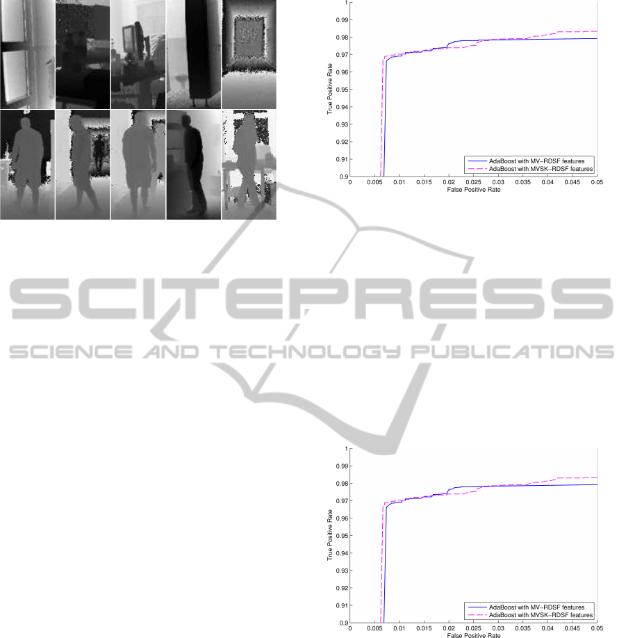
Figure 4: The upper part of the figure includes negative ex-
amples of the training and test set and the lower part of the
figure shows some positive examples.
described in (Ikemura and Fujiyoshi, 2010), is not in
focus of this evaluation, the positive examples include
only small partial occlusion from the foreground and a
large variation of the background, including also am-
biguities in the depth caused by the time of flight prin-
ciple.
5.2 Feature Performance Comparison
The evaluated classical HOG features contain one cell
((8 × 8) pixel) per block to be comparable to the new
combined MV-HOG-RDSF. Each possible rectangu-
lar region from (8 × 8) pixel up to (56 × 112) pixel
with an increasing factor of 8 pixel in each dimension
of the block will be considered. Additionally, each
possible HOG block will be shifted by one pixel over
the whole training window, as described also in sec-
tion 3, and not by the smallest cell size as it will be
done by the RDSFs. This results in a total number of
48510 classical HOG features.
Figure 5 shows the results of the trained classi-
fiers with the new features based on mean, variance,
skewness and kurtosis. The mean and variance fea-
tures (MV-RDSF) deliver the worst performance. By
extending the MV-RDSF with skewness and kurtosis
properties, it is possible to increase the performance
of the classifier only slightly. However, both features,
the MV-RDSF and the MVSK-RDSF, cannot reach
the performance of the original RDSF, because the
feature space is strongly limited for a good separa-
tion. Strong noise involved by the depth ambiguity
and the sensor hardware cannot be considered just by
the mean and variance of depth information.
The comparison between the classical HOG fea-
ture and the RDSF of (Ikemura and Fujiyoshi, 2010)
is shown in Figure 6. The classical HOG feature
has similar results as the RDSF of (Ikemura and Fu-
Figure 5: The receiver operating characteristics (ROCs) of
the MV-RDSF and MVSK-RDSF trained with the asym-
metric AdaBoost procedure.
jiyoshi, 2010). Again, it is mentionable that in (Ike-
mura and Fujiyoshi, 2010) it is not described which
version of a HOG feature has been used. Here, as
described in section 3, one HOG block consists of
one cell with the size of (8 × 8) pixel and has only
5 orientations. The concatenation of the MV-RDSF
and the HOG features, the MV-HOG-RDSF, uses a
combination of similarity in depth and depth gradi-
ents for shape characterization and delivers the best
results in the experiments, as it can be seen in Figure
6. Based on the LDA transformation of the combined
Figure 6: The receiver operating characteristics (ROCs) of
the classical HOG feature, the RDSF and the MV-HOG-
RDSF trained with the asymmetric AdaBoost procedure.
depth relation and depth gradients, more information
for the separation of positive and negative examples
are available. On the other hand, the computation of
the integral images for the orientations of the classical
HOG feature and the integral images over the mean
and variance of the depth image is still faster than the
generation of 25 integral images to quantize the depth
image as used by (Ikemura and Fujiyoshi, 2010). Fur-
thermore, the calculation of the MV-HOG-RDSF in
the online detection phase is still faster than the com-
putation of the RDSF, because for each RDSF the
VISAPP2015-InternationalConferenceonComputerVisionTheoryandApplications
354

Bhattacharyya distance of two 25 dimensional vec-
tors has to be determined. This improvement in speed
and the better performance in detection favour the us-
age of the MV-HOG-RDSF for the human detection
in depth images, where strong occlusion of the hu-
mans has not to be considered.
Each classifier has been trained with a final false
positive rate of 1%. To compare the performance of
the different features, the 1% false positive point on
the ROC curves will be used. Table 1 includes the re-
sults of the ROC curves in this point for each feature
used with the asymmetric AdaBoost classifier. The
Table 1: The table inlcudes the results of the different fea-
tures at the 1% false positive point on the ROC curves. The
last column shows the number of selected features of the
final classifier which has been selected during the training
phase.
Feature True Positive Rate Number of Features
MV-RDSF 0.9703 73
MVSK-RDSF 0.9703 103
MV-HOG-RDSF 0.9867 24
Classic HOG 0.9811 33
RDSF 0.9828 41
MV-RDSF and MVSK-RDSF are significantly infe-
rior to the RDSF, but the combination of gradients
features and depth features deliver an improved de-
tection accuracy.
5.3 Relative Time Performance
However, the gap in the performance is not so large,
but the time complexity of the feature and integral im-
age calculation between the RDSF and the MV-HOG-
RDSF is huge. The calculation of the integral im-
ages of the MV-HOG-RDSF is twice as fast as of the
RDSF, without pronouncing the absolute time values,
which are hardware dependent. It is worthwhile to
know, no parallelization has been used for each com-
putation. Additionally, the single feature calculation
of the MV-HOG-RDSF is also still faster than the cal-
culation of the Bhattacharyya distance between two
25 dimensional feature vectors.
Furthermore, the computational costs of the final
classifiers are directly dependent from the number of
selected features in the training procedure. As it can
be seen in Table 1, the MV-RDSF and MVSK-RDSF
have many selected features in the final classifier, but
are still very fast due to the simplicity of the used fea-
tures. The new MV-HOG-RDSF have just almost half
of the number of selected features for the final classi-
fier as the RDSF and also less selected features than
the classical HOG features. The reduced number of
selected features and the low computational complex-
ity of the MV-HOG-RDSF in relation to the RDSF
(a) True positive examples hallway
(b) True positive example room
(c) True and false positive examples
Figure 7: Subfigure 7(a) shows some true positive results
of the MV-HOG-RDSF classifier in a hallway, where depth
ambiguities can occur. Subfigure 7(b) includes a true posi-
tive example in a room without the presence of depth ambi-
guities and in subfigure 7(c) are a true positive and a false
positive example visible, where the false positive example
is influenced by depth ambiguity.
LDACombinedDepthSimilarityandGradientFeaturesforHumanDetectionusingaTime-of-FlightSensor
355

shows the excellent usage of the LDA combination of
depth similarity and gradient features for human de-
tection in depth images.
6 CONCLUSIONS
To reduce the complexity of the RDSF calculation
and to keep the performance just by usage of mean
and variance features on the depth image, delivers not
sufficiently accurate results. The computational time
of the MV-RDSF is very fast, but the accuracy of the
original RDSF cannot be reached. Since, the feature
space of the MV-RDSF is not significantly enough to
separate the dataset, a LDA combination between the
classical HOG feature and the MV-RDSF shows very
good attributes to solve the problem. The time com-
plexity of the MV-HOG-RDSF is better than of the
RDSF (Ikemura and Fujiyoshi, 2010) and less fea-
tures are selected (needed) in the training to separate
the positive examples from the negative ones. Fur-
thermore, just the depth image, and not the intensity
or the RGB image, is needed, for a good classifica-
tion result. The complexity of computing the inte-
gral images and features add up to a fast classification.
Based on the LDA combination, just one classifier is
needed and not a decision fusion of different classi-
fiers, which are using just one of both feature types,
as it has been done in (Wang et al., 2012).
Further research could try to combine other depth
features with each other to reach more and more
the best possible classification result. Still on focus
should be the time complexity of the used features to
produce as fast as possible classifiers for real time ap-
plications, where real time means to ensure the com-
putation of all methods inside the frame rate of the
underlying sensor, in this case 33ms.
ACKNOWLEDGEMENT
The research of the project ”Move and See” leading
to these results has received funding from the Min-
istry of Health, Equalities, Care and Ageing of North
Rhine-Westphalia (MGEPA), Germany and the Euro-
pean Union.
REFERENCES
Dalal, N. and Triggs, B. (2005). Histograms of Oriented
Gradients for Human Detection. In Proceedings of
the IEEE Computer Society Conference on Computer
Vision and Pattern Recognition (CVPR’05), volume 1,
pages 886–893, San Diego,California,USA.
Doll
´
ar, P., Wojek, C., Schiele, B., and Perona, P. (2012).
Pedestrian Detection: An Evaluation of the State of
the Art. IEEE Transactions on Pattern Analysis and
Machine Learning, 34(4):743 – 761.
Enzweiler, M. and Gavrila, D. M. (2009). Monocular
Pedestrian Detection: Survey and Experiments. IEEE
Transactions on Pattern Analysis and Machine Intel-
ligence, 31(12):2179 – 2195.
Ikemura, S. and Fujiyoshi, H. (2010). Real-Time Hu-
man Detection using Relational Depth Similarity Fea-
tures. In Proceedings of the 10th Asian Conference on
Computer Vision (ACCV’10), pages 25 – 38, Queen-
stown,New Zealand.
Izenman, A. J. (2008). Modern Multivariate Statistical
Techniques - Regression, Classification, and Manifold
Learning. Springer New York.
Keller, C. G., Enzweiler, M., and Gavrila, D. M. (2011). A
New Benchmark for Stereo-Based Pedestrian Detec-
tion. In IEEE Intelligent Vehicles Symposium (IV’11),
pages 691 – 696, Baden-Baden,Germany.
Mattheij, R., Postma, E., van den Hurk, Y., and Spronck,
P. (2012). Depth-based detection using haar-like fea-
tures. In Proceedings of the 24th BENELUX Confer-
ence on Artificial Intelligence (BNAIC’12), pages 162
– 169, Maastricht,Netherlands.
Nunn, C., M
¨
uller, D., Meuter, M., M
¨
uller-Schneiders,
S., and Kummert, A. (2009). An Improved Ad-
aboost Learning Scheme using Lda Features for Ob-
ject Recognition. In Proceedings of the 12th In-
ternational IEEE Conference on Intelligent Trans-
portation Systems (ITSC’09), pages 486 – 491, St.
Louis,MO,USA.
Shafait, F., Keysers, D., and Breuel, T. M. (2008). Effi-
cient Implementation of Local Adaptive Threshold-
ing Techniques Using Integral Images. In Yanikoglu,
B. A. and Berkner, K., editors, Proceedings SPIE
6815,Document Recognition and Retrieval XV.
Spinello, L. and Arras, K. O. (2011). People detection
in RGB-D data. In Proceedings of the IEEE/RSJ
International Conference on Intelligent Robots and
Systems (IROS’11), pages 3838 – 3843, San Fran-
cisco,CA,USA.
Viola, P. and Jones, M. (2001a). Fast and Robust Classi-
fication using Asymmetric AdaBoost and a Detector
Cascade. In Advances in Neural Information Process-
ing System 14, pages 1311 – 1318. MIT Press.
Viola, P. and Jones, M. (2001b). Rapid Object Detection
Using a Boosted Cascade of Simple Features. In Pro-
ceedings of the IEEE Computer Society Conference on
Computer Vision and Pattern Recognition (CVPR’01),
volume 1, pages 511 – 518, Kauai,HI,USA.
Wang, N., Gong, X., and Liu, J. (2012). A New Depth
Descriptor for Pedestrian Detection in RGB-D Im-
ages. In Proceedings of the 21st International Confer-
ence on Pattern Recognition (ICPR’12), pages 3688 –
3691, Tsukuba,Japan.
Wu, S., Yu, S., and Chen, W. (2011). An attempt to pedes-
trian detection in depth images. In Proccedings of the
3rd Chinese Conference on Intelligent Visual Surveil-
lance (IVS’11), pages 97 – 100, Beijing,China.
VISAPP2015-InternationalConferenceonComputerVisionTheoryandApplications
356
