A Comparison between Multi-Layer Perceptrons and Convolutional

Neural Networks for Text Image Super-Resolution

ement Peyrard

1,2

, Franck Mamalet

and Christophe Garcia

Orange Labs, 4 rue du Clos Courtel, 35512 Cesson-S

evign

e, France

LIRIS, INSA Lyon, 20 avenue Albert Einstein, Villeurbanne, France

Keywords:

Super-Resolution, Text Image, Multi-Layer Perceptron, Convolutional Neural Network, OCR.

Abstract:

We compare the performances of several Multi-Layer Perceptrons (MLPs) and Convolutional Neural Net-

works (ConvNets) for single text image Super-Resolution. We propose an example-based framework for both

MLP and ConvNet, where a non-linear mapping between pairs of patches and high-frequency pixel values is

learned. We then demonstrate that for equivalent complexity, ConvNets are better than MLPs at predicting

missing details in upsampled text images. To evaluate the performances, we make use of a recent database

(ULR-textSISR-2013a) along with different quality measures. We show that the proposed methods outper-

forms sparse coding-based methods for this database.

1 INTRODUCTION

Super-Resolution (SR) methods aim to provide a

high-deﬁnition image from one or several low resolu-

tion (LR) images. With the increasing quantity of vi-

sual data due to advances in information technologies

and portable devices, these methods have been exten-

sively studied in the last decades. SR can ensure a

better visual experience for HD displays or visual ap-

peal in videos or photographs, but also improve the re-

sults of automated resolution-dependent vision tasks

such as face recognition/detection or optical character

recognition (OCR), if used as a pre-processing step.

SR techniques can be divided into several cate-

gories. (Nasrollahi and Moeslund, 2014) provides a

complete overview of the existing methods, according

to the available single or multiple LR images. Mul-

tiple image Super-Resolution takes advantage of the

redundancy of the information in the different image

representing the same scene to merge this low res-

olution information into a high resolution (HR) im-

age after an alignment process. Several techniques

have been introduced such as Iterative Back Projec-

tions (Irani and Peleg, 1991), Projection Onto Convex

Sets (Stark and Oskoui, 1989), Maximum Likelihood

and Maximum A Posteriori (Cheeseman et al., 1996).

For Single Image Super-Resolution (SISR), the task

is of another nature as we only have one representa-

tion of the original scene. The recovery of the original

high-resolution is a drastically ill-posed inverse prob-

lem, and the details lost during the down-sampling

process might only be reﬁned either by processing

an up-sampled version of the LR image (interpolation

or reconstruction based methods, such as (Sun et al.,

2011)), or by training a system on some external data

(Freeman et al., 2002) to hallucinate high-resolution

information from a LR one (learning-based methods).

More speciﬁcally, Text Image SR – also referred

to as Text Document SR – has been handle in dif-

ferent ways. Several methods have been proposed

or applied for multiple images (Donaldson and My-

ers, 2005; Mancas-Thillou et al., 2005; Protter et al.,

2009). For the task of Single Images, (Thouin and

Chang, 2000) used an iterative method to minimize

a Bimodal-Smoothness-Average score, (Dalley et al.,

2004) adopted a bayesian approach for SR of binary

text images. (Luong and Philips, 2007) proposed a

non-local search to take advantage of characters re-

dundancies in documents. (Zheng et al., 2014) pro-

posed a fast matting technique that consists in ex-

tracting and interpolate foreground, background and

a matte (proportion of foreground/background), and

enhance the matte layer with a Teager Filter before

using it to mix the foreground and background layers

back together.

Most recent and successful text image are learn-

ing based ones, and this paper will start with a short

survey in 2. We then express the SR problem in 3

and depict our proposal in 4. We describe our ex-

perimentations in 5 and present the obtained results.

Peyrard C., Mamalet F. and Garcia C..

A Comparison between Multi-Layer Perceptrons and Convolutional Neural Networks for Text Image Super-Resolution.

DOI: 10.5220/0005297200840091

In Proceedings of the 10th International Conference on Computer Vision Theory and Applications (VISAPP-2015), pages 84-91

ISBN: 978-989-758-089-5

 2015 SCITEPRESS (Science and Technology Publications, Lda.)

Conclusion and perspectives are ﬁnally given in 6.

2 LEARNING-BASED METHODS

FOR SUPER-RESOLUTION

We provide a quick review of some learning-based

methods for SISR.

2.1 Dictionnary Training and Sparse

Coding

Different learning framework have already been pro-

posed in the literature. Authors successively proposed

to learn dictionaries of LR/HR patch pairs called D

and D

, and reconstruct a SR image from a mixture

of the HR versions of the closest LR patches. (Free-

man et al., 2002) ﬁrst proposed to look up for the 16

nearest neighbours in a dictionary and keep the high

patches showing a good spatial compatibility on over-

lapping region. A similar method have been applied

by(Fan et al., 2012) on text images. (Glasner et al.,

2009) set up a intra-image dictionary to take advan-

tage of the redundant structures inside an image at

different positions and scales. These methods exhibits

very good results given an image with redundancy

and a known Point Spread Function for the decima-

tion process.

Later, in (Yang et al., 2010; Walha et al., 2012),

authors proposed to ﬁnd the best sparse representa-

tion of a feature vector y in D

(called

α) for the min-

imization problem:

α = argmin

y − D

+ λ

(1)

so that one can reconstruct the HR version of the cur-

rent patch with the same sparse

α, but using D

. To

ensure sparsity on

α, a regularization parameter is

added, here using `

norm. Note that in (Yang et al.,

2012) and (Peleg and Elad, 2014), Neural Networks

are used to speed up the choice of the sparse vector

α. In (Timofte et al., 2013), this speed-up is done by

pre-computing a neighbourhood for each atom in the

dictionary.

2.2 Autoencoders

With the recent work on autoencoding architectures,

two different approaches were proposed to take ad-

vantage of autoencoders for SR. The ﬁrst one (Gao

et al., 2013) is strongly related to sparse coding meth-

ods. It encodes a dictionary of LR/HR patch pairs in a

Restricted Boltzmann Machine and take advantage of

the RBM framework to iteratively reconstruct an HR

image as a sparse mixture of the embedded patches,

via a sparse activation of hidden neurons. The second

(Nakashika et al., 2013) makes use of a Deep Belief

Network to learn the autoencoding of the DCT coef-

ﬁcients of HR images. Then, from the low-frequency

coefﬁcient of a scaled-up LR image, the network iter-

atively recovers high-frequency as it is the only kind

of image it has learned to produce. (Peleg and Elad,

2014) also use a RBM to encode a relationship be-

tween sparse representations in overcomplete dictio-

naries.

2.3 Artiﬁcial Neural-networks Based

Methods

ANN are architectures inspired from the human brain.

They interconnect cells that perform a non-linear

mapping between their weighted inputs (”dendrites”)

and their output (”axone”). The Perceptron model

was ﬁrst introduced by (Rosenblatt, 1958) to model

human neurons. It applies a non-linear function Φ

(such as tanh) to the weighted sum of its inputs (see

1).

y = Φ

bias

∑

i=1

(2)





































…

Figure 1: Perceptron Model.

ANN for SR were introduced in (Ahmed et al.,

1995; Plaziac, 1999), where they proposed to take ad-

vantage of a neural networks to handle interpolation

problems: how to choose the best missing pixel be-

tween existing pixels. Later, (Pan and Zhang, 2003)

successfully applied a neural network design to es-

timate residual errors in an HR estimate from the

ones in LR on natural and text images. The ﬁrst

model presented in this paper is related to their as we

want to automatically learn how to infer missing de-

tails. (Panagiotopoulou and Anastassopoulos, 2007)

trained a network successively using examples at dif-

ferent scales for scanned document SR. (Carcenac,

2007) proposed a Neural Network architecture for

face image super-resolution. Recently, (Dong et al.,

2014) proposed a Deep Convolutional Neural Net-

work, that maps an interpolated image to its HR coun-

terpart. A ﬁrst layer is employed to extract features

AComparisonbetweenMulti-LayerPerceptronsandConvolutionalNeuralNetworksforTextImageSuper-Resolution

maps, which are non-linearly mapped onto a second

layer of feature maps of the same size. Finally, a fu-

sion of the maps is performed by a single fully con-

nected convolution.

In the present work, we compare two neural based

approaches and favour a high frequency restoration

scheme rather than an intensity based one.

3 PROBLEM FORMULATION

We model the SR problem by a reconstruction pro-

cess. Given an HR image x and its LR counterpart

y, we want to infer the missing details in an upscaled

version of the LR image. Therefore, we choose a sim-

ple interpolation method (e.g. bicubic) that produces

an estimate

bic

of the SR image. This estimate is

often smooth, blurry, and may also present ringing ar-

tifacts.

At each position (k,l) of an image, the estimate

bic

(k, l) differs from the original (or ideal HR) image

x(k, l) by an error e(k, l), deﬁned as:

e(k, l) = x (k, l)−

bic

(k, l) (3)

the estimate

bic

being the upscaled version of the

original LR image:

bic

= f

(y) (4)

with an interpolation function f

. Therefore, we want

a SR system to be able to provide an estimate

e(k, l)

of this difference. This difference can be considered

as high spatial frequency information, as the interpo-

lated image gives a smooth version of the desired HR

image. The reconstruction process is then:

bic

e (5)

In the next section, we present the set up of two

neural-based architectures able to provide this esti-

mate.

4 PROPOSED METHODS

In this paper, we aim to compare two neural networks

models for the SR problem. For both, the framework

is the same: a network takes as input a LR patch ex-

tracted from y, and targets, for a given scale factor

s, s

output values that correspond to the estimate

e for each s

central pixel in the corresponding SR

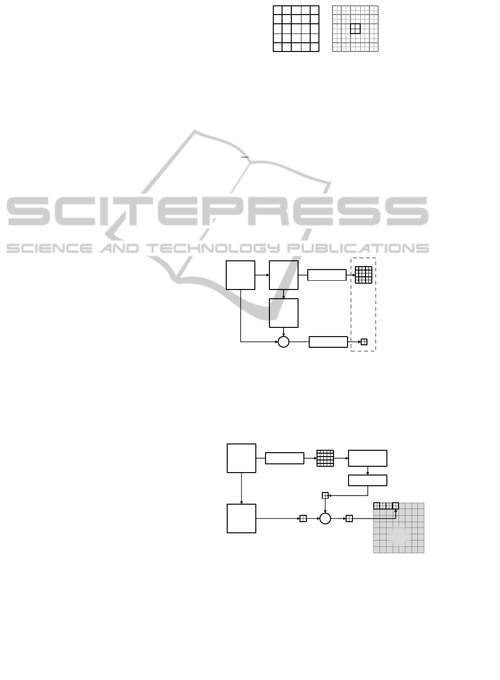
patch (see 2). We also wish to limit the complexity

of the networks, i.e. restrict the number of weights

to be learned to differentiate from deep learning ap-

proaches.

Figure 2: Representation of a LR patch (left) and the

= 4 central pixels (for a scale factor of two).

To train these networks, we start with collecting

pairs of LR patch and corresponding s

reconstruc-

tion errors (see 3). The weights of the neural networks

are classically trained using a backpropagagtion algo-

rithm with momentum to lower the mean square error

E =

∑

(

e − e)

A simple normalization is applied to the input

patches by subtracting the central pixel value of the

LR patch, and dividing by a constant K

. The s

out-

puts correspond to the missing details between the s

ground truth pixel and the s

upsampled pixels ob-

tained by the interpolation method. They are normal-

ized by a pre-determined constant K

out

as well.

Image

Bicubic

Image

Input Patch

Target Upsampling

Residual Error

Pair

Extraction

Normalization

Figure 3: Training dataset construction

(for 5×5 input patch and a scale factor s = 2).

At reconstruction (4), overlapping patches are ex-

tracted, and the estimated high-frequency details are

added to the interpolated image

bic

Image

Bicubic

Image

Normalization

Trained Neural

Network

















Image

Figure 4: Reconstruction scheme for a SR image

(represented for 5 × 5 input patch, s = 2 scale factor).

A classical alternative for input patches is to use

VISAPP2015-InternationalConferenceonComputerVisionTheoryandApplications

an upscaled version of the patches (extracted from

bic

for instance) to spread the information onto a wider

input area. The problem would get closer to a deblur-

ring one, but is still part of a SR approach as we origi-

nally rely on an interpolation method, which only de-

pends on some LR data and cannot be properly mod-

elled with a blurring kernel or a degradation model.

Here, we decided to keep the original LR information,

as it holds all the available information while keeping

reasonable dimensions for the input data.

4.1 Multi-Layer Perceptron

As stated in the previous paragraph, this method is

quite similar to the one described in (Pan and Zhang,

2003), but the direct use of pixel intensity to predict

details has not been exploited to the best of our knowl-

edge. We design a MLP with N

neurons for the in-

put layer and s

linear neurons for the output layer.

The N

inputs correspond to a N × N patch. Most

…

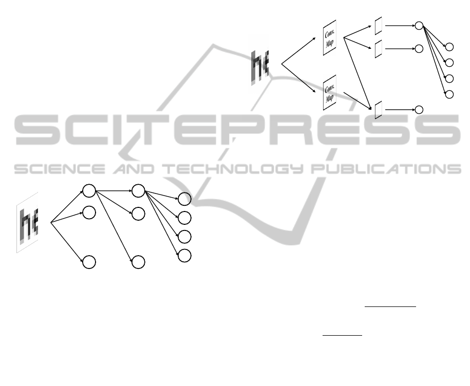
Input Layer

Hidden

Layer

Output

Layer

…

Hidden

Layer

Figure 5: Proposed MLP architecture for SR.

approaches in the literature only make use of one

hidden-layer for SR with MLP. We noted that two hid-

den layers, with respectively N

and N

neurons per

layer with tanh activation function, were more likely

able to capture the non linearity of the input-target

mapping. However, this increases the complexity of

the network.

4.2 Convolutional Neural Network

ConvNets (LeCun and Bengio, 1995) are biologically

inspired neural architectures that include several con-

volutional layers in the network. They can be consid-

ered as feature detectors that keep track of the spatial

position of those features, producing a set of feature

maps at each layer. The strength of this architecture

is that convolution kernels are learnt using backprop-

agation, leading to an optimal solution compared with

hand-crafted ﬁlters.

In classiﬁcation, one can add pooling layers (orig-

inally called downsampling layers), when the precise

position of features is not crucial. For the SR prob-

lem, however, the spatial location of a feature in the

image is very important, and pooling, if used, should

be handled with care. Our experiments in this pa-

per do not involve any pooling layer, as simple test

demonstrated that the result do not beneﬁt from such

layers.

…

Input Layer

(patch)

Output

Layer

Hidden

Layer

…

Figure 6: Proposed ConvNet architecture for SR.

We propose to use the following architecture: the

LR patch at the input layer is convolved with N

ker-

nels, producing N

maps for the ﬁrst layer C1. Each

of these maps are then convolved with a second set of

kernels following the same connection scheme as

the one presented in (Garcia and Delakis, 2004). Each

map in C1 is convolved by two dedicated kernels to

foster specialization, giving a ﬁrst subset of 2 × N

kernels for C2. In parallel, fusion is also performed

convolving each possible pair of maps of C1 by a ker-

nel, which gives another





kernels. Therefore we

have:

= (2 × N

) +



− 2)!2!



= N

+ 3)

(6)

We add a hidden layer of N

neurons, each of which

is connected to a single map, non-linearly merging

the information of the last maps into a single output

value that is presented to the output layer. The out-

put layer consists in s

fully connected linear neurons.

Note that all the previous layers include tanh activa-

tion function. We train this network with our set of

patch and target pairs, using backpropagation to si-

multaneously learn the weights of the neurons and the

kernels of the convolutions.

5 EXPERIMENTAL RESULTS

To compare the performances of our proposed ap-

proaches, we use the text image database ULR-

textSISR-2013a released by (Nayef et al., 2014). The

AComparisonbetweenMulti-LayerPerceptronsandConvolutionalNeuralNetworksforTextImageSuper-Resolution

test set contained in this database consists in 30

grayscale images of black text over a white back-

ground: 5 different texts, each rendered with 3 differ-

ent fonts (Arial, Times, Courier) and 2 different sizes

(10 and 12 pt, at 150dpi), using anti-aliasing ﬁlters

during Portable Document Format (PDF) ﬁle genera-

tion. They contain bold and italic characters.

5.1 Evaluation Procedure: Measures

We use the same measure as (Nayef et al., 2014) to

evaluate the performances of the different proposed

methods: Mean Squared Error (MSE), Peak Signal to

Noise Ration (PSNR), OCR accuracy.

1. MSE reﬂects the squared difference in gray lev-

els between two images. Its square root (RMSE)

gives the standard error (in graylevel), indicating

the average error obtained in our reconstruction.

2. Employed in signal processing, PNSR give a more

absolute meaning to the reconstruction, given the

maximum value the signal can reach. It is still

closely related to the MSE.

PSNR = 10 × log



255

MSE



3. When processing text images we can produce a

joint evaluation of both standard measures and

classiﬁcation, recognition or detection scores.

Optical Character Recognition systems allow

to produce an accuracy measure for evaluation

(which is the Levenstein distance between recog-

nized characters and ground truth transcription,

divided by the total number of characters). Fol-

lowing the proposal of (Nayef et al., 2014), we

evaluate our performances of our using the same

tools (Tesseract OCR 3.02 and UNLV-ISRI accu-

racy tool). The results do not take into account

ground truth spacing characters, although includ-

ing the related errors.

5.2 Settings

5.2.1 Framework Global Settings

Normalization. We set K

= 256 to normalize the

input patch from which we subtract the central value.

This way, we ensure that values range from −1 to 1.

For output detail pixels, we choose K

out

= 100 for im-

ages of black text over a white background, which is

out

' ν with ν being the variance of the histogram of

target values in the training dataset.

Patch Size. In order to provide an equivalent evalu-

ation of the two methods, we try to use an equivalent

amount of information at the entrance of both sys-

tems. For ConvNets, we use 9×9 LR patches. Tak-

ing into account the border effect of convolutions in

the ﬁrst layers, we consider that presenting only 7×7

patches to the MLP is equivalent in terms of informa-

tion. Experiments show that the MLP does not beneﬁt

from larger patches.

Scale. In this study, we only consider ×2 SR since

the database (Nayef et al., 2014) was provided for this

upsampling factor, although our implementation can

handle higher scale factors (the output layers would

be 3×3 for ×3 SR, 4×4 for ×4 SR, etc.)

Training Database. For training, we use text im-

ages generated with the process employed to build the

database (Nayef et al., 2014): Times and Arial fonts

(10 and 12pt at 150dpi), bold, italic and normal em-

phasis; FreeType generation and Matlab downsam-

pling. An interesting aspect of this database is that it

includes three different fonts (Arial, Times, Courier)

in the test data while only two of them are present in

the training data. This allows to evaluate if the SR

method generalizes to text of different nature.

We extract 120,000 pairs for training as described

in 3. We simply reject strictly uniform input patches

(typically, white patches).

5.2.2 Performance Evaluation of the MLP

We evaluated with different numbers of neurons per

hidden layer and tried to outline a global trend (see

1). For each conﬁguration, we run 100 epochs over

the whole set of pairs, with a constant learning rate

λ = 10

−3

and a momentum of 0.2. Generally, the re-

sults get better with an increasing number of neurons,

but it also depends on the repartition of the weights

and how N

is related to N

. However, the con-

ﬁguration seems to reach its limits and at a certain

point and increasing the complexity of the network

does not improve the performances. The best perfor-

mances are obtained for a network with 100 neurons

in N1, and 150 neurons in N2 layers (conﬁguration 6,

20,754 weights).

5.2.3 Performance Evaluation of the ConvNet

To choose the most interesting network dimensions

for our purpose, and given the chosen architecture

(4.2), we tested several ConvNet sizes as reported in

2. For each conﬁguration, we use 5×5 kernels for

C1 and 3×3 kernels for C2. We can notice that small

networks with N

as small as conﬁgurations 2 or 3

VISAPP2015-InternationalConferenceonComputerVisionTheoryandApplications

Table 1: Performances of different MLP conﬁgurations.

Conﬁg. 1 2 3 4 5 6 7

N1-N2 10-10 10-50 50-50 50-100 50-150 100-150 100-200

Complex. 654 1,254 5,254 8,004 10,754 20,754 26,004

PSNR 22.01 22.67 23.05 23.25 23.63 24.15 24.05

MSE 20.52 19.03 18.20 17.80 17.05 16.03 16.23

OCR 91.97 93.28 92.85 93.73 93.82 94.69 94.44

Table 2: Performances of different ConvNet conﬁgurations.

Conﬁg. 1 2 3 4 5 6 7 8 9 10

C1 2 4 8 12 16 20 24 28 32 40

Complex. 185 498 1,520 3,070 5,148 7,754 10,888 14,550 18,740 28,704

PSNR (dB) 20.49 21.59 22.89 23.25 23.88 23.79 24.18 24.16 24.55 24.48

MSE 24.36 21.51 18.48 17.74 16.47 16.67 15.91 15.95 15.27 15.39

OCR (%) 90.35 90.70 93.35 95.08 95.23 95.10 95.49 96.09 96.42 96.13

perform well with less than 2,000 weights. The ar-

chitecture reaches its limits for N

= 32 which has

18,740 weights.

As mentioned before, we tried to limit the size

of the network. We also explored larger networks

where the hidden layer was fully connected, increas-

ing drastically the complexity up to 481,784 weights.

They allow to reach higher scores (25.69 dB / 13.58

/ 96.67%) but are out of the scope of the desired low

complexity.

5.3 Results

For the selected architectures, we can observe in 1 and

2 the advantage of ConvNets compared with MLP.

For an equivalent complexity (e.g. around 20, 000

weights), ConvNets produces a better version of miss-

ing high-frequencies, improving both pixel-wise mea-

sures (PSNR from 24.15 to 24.55 dB) and OCR score

(94.69 to 96.44%). Some results are shown in ﬁgures

7(b) and 7(c).

The bicubic image (7(a)) exhibits serious blur ar-

tifacts, and the gain of the proposed Neural-based

methods is clear. Moreover, we can note a better

reconstruction of some sensitive details for the Con-

vNets: holes in the ”e” letters are more visible, ”s”

letters are better shaped, and some ﬁne edges such as

”n”, ”k” or ”g” curves are more nicely reconstructed.

We report in 3 the state of the art results published

on this database, and compare them with our best re-

sults. We can see the beneﬁt of our method over the

sparse coding methods for both pixel-wise measures

and OCR accuracy score. We observe a gain for MLP

and ConvNet, of respectively +4.46 dB and +4.86

dB for PSNR, and +1.10% and +2.85% for OCR ac-

curacy.

(a) Bicubic interpolation

(b) MLP result

Figure 7: Bicubic and Super-resolved test image.

Table 3: Proposed methods performances compared with

State-of-the-Art ones.

Method RMSE PSNR (dB) OCR (%)

Bicubic 34.92 17.32 88.57

Yang 26.75 19.69 93.59

Walha 29.45 18.82 93.16

MLPTextSR 16.03 24.15 94.69

CNNTextSR 15.27 24.55 96.44

Original HR - - 97.86

Supplementary Experiments

The proposed database is very speciﬁc as it only con-

tains text images with black font over a white back-

AComparisonbetweenMulti-LayerPerceptronsandConvolutionalNeuralNetworksforTextImageSuper-Resolution

Table 4: PSNR scores for ”Set5”.

Bicubic ANR SRCNN Our (7×7) Our (9×9)

baby 37.07 38.44 38.3 37.92 37.96

bird 36.81 40.04 40.64 40.23 40.32

butterﬂy 27.43 30.48 32.2 31.63 31.66

head 34.86 35.66 35.64 35.47 35.48

woman 32.14 34.55 34.94 34.64 34.63

(a) Bicubic (b) ANR (c) SRCNN (d) Our method 9×9 (e) Groundtruth

Figure 8: Results for natural images (×2).

ground. Thus, for the sake of generalization, we tried

our system on natural images. We use the same data

as (Dong et al., 2014) or (Yang et al., 2010) for train-

ing, and images extracted from BSD100 segmentation

database for validation. The test dataset is ”Set5”. We

tried to preserve fairness with the other methods. As

(Dong et al., 2014) use 24,800 32×32 subimages for

training their system while we use patches (7×7 or

9×9 for this last experiment), we consider that we can

randomly extract 2,000 patches from each of the 92

training images without turning into a deeper learn-

ing process than they do. In terms of complexity, their

system contains W = 8, 032 weights. Using N

= 20

for both 7×7 and 9×9 patch sizes, we end up with re-

spectively W

7×7

= 7, 434 and W

9×9

= 7, 754. We use

the same setting as 5.2.3, except for 3×3 convolutions

for all convolutions in the 7×7 input patches case.

Our results (4 and 8) are competitive with the recent

methods applied on this dataset: Anchored Neighbour

Regression (Timofte et al., 2013) and SRCNN (Dong

et al., 2014).

6 CONCLUSIONS AND

PERSPECTIVES

We compared two neural network based methods

and demonstrated the efﬁciency of reasonably sim-

ple Convolutional Networks to provide super resolved

single text images via a good estimate of missing de-

tails from overlapping patches of their low resolution

version. Furthermore, we observed better results than

the proposed state-of-the-art sparse coding methods.

The experiments on natural images demonstrated that

the proposed ConvNet architecture can be generalized

to other types of images.

These results motivate further research: take

advantage of recent proposed architectures for

ConvNets in SR to enhance our model, confront our

system to noisy contexts where patch-based method

usually perform well at denoising and adapt it to dif-

ferent kinds of images such as overlaid text in TV

streams.

REFERENCES

Ahmed, F., Gustafson, S., and Karim, M. (1995). High-

ﬁdelity image interpolation using radial basis function

neural networks. In Proceedings of the IEEE 1995

National Aerospace and Electronics Conference, vol-

ume 2, pages 588–592.

Carcenac, M. (2007). A modular neural network for

super-resolution of human faces. Applied Intelligence,

30(2):168–186.

Cheeseman, P., Kanefsky, B., Kraft, R., Stutz, J., and Han-

son, R. (1996). Super-resolved surface reconstruc-

tion from multiple images. In Maximum Entropy and

Bayesian Methods, pages 293–308. Springer.

Dalley, G., Freeman, B., and Marks, J. (2004). Single-frame

text super-resolution: a bayesian approach. In Inter-

national Conference on Image Processing, volume 5,

pages 3295–3298 Vol. 5.

Donaldson, K. and Myers, G. (2005). Bayesian Super-

Resolution of Text in Video with a Text-Speciﬁc Bi-

modal Prior. IEEE Computer Society Conference on

Computer Vision and Pattern Recognition, 1:1188–

1195.

Dong, C., Loy, C. C., He, K., and Tang, X. (2014). Learn-

ing a deep convolutional network for image super-

resolution. In Computer Vision–ECCV 2014, pages

184–199. Springer.

VISAPP2015-InternationalConferenceonComputerVisionTheoryandApplications

Fan, W., Sun, J., Naoi, S., Minagawa, A., and Hotta,

Y. (2012). Local Consistency Constrained Adap-

tive Neighbor Embedding for Text Image Super-

Resolution. 10th IAPR International Workshop on

Document Analysis Systems, pages 90–94.

Freeman, W., Jones, T., and Pasztor, E. (2002). Example-

based super-resolution. Computer Graphics and Ap-

plications, IEEE, 22(2):56–65.

Gao, J., Guo, Y., and Yin, M. (2013). Restricted boltzmann

machine approach to couple dictionary training for

image super-resolution. In IEEE International Con-

ference on Image Processing, pages 499–503.

Garcia, C. and Delakis, M. (2004). Convolutional face

ﬁnder: A neural architecture for fast and robust face

detection. IEEE Transactions on Pattern Analysis and

Machine Intelligence, 26(11):1408–1423.

Glasner, D., Bagon, S., and Irani, M. (2009). Super-

resolution from a single image. IEEE 12th Interna-

tional Conference on Computer Vision, pages 349–

356.

Irani, M. and Peleg, S. (1991). Improving resolution by im-

age registration. CVGIP: Graph. Models Image Pro-

cess., 53(3):231–239.

LeCun, Y. and Bengio, Y. (1995). Convolutional networks

for images, speech, and time series. The handbook of

brain theory and neural networks, 3361.

Luong, H. Q. and Philips, W. (2007). Non-local text image

reconstruction. In Ninth International Conference on

Document Analysis and Recognition, volume 1, pages

546–550.

Mancas-Thillou, C., Mirmehdi, M., and Copernic, A.

(2005). Super-resolution text using the teager ﬁlter.

First International Workshop on Camera-Based Doc-

ument Analysis and Recognition, pages 10–16.

Nakashika, T., Takiguchi, T., and Ariki, Y. (2013). High-

Frequency Restoration Using Deep Belief Nets for

Super-resolution. International Conference on Signal-

Image Technology & Internet-Based Systems, pages

38–42.

Nasrollahi, K. and Moeslund, T. (2014). Super-resolution:

a comprehensive survey. Machine Vision and Appli-

cations, 25(6):1423–1468.

Nayef, N., Chazalon, J., Gomez-Kr

amer, P., and Ogier, J.

(2014). Efﬁcient example-based super-resolution of

single text images based on s elective patch process-

ing. In 11th International Workshop on Document

Analysis Systems, pages 227–231.

Pan, F. and Zhang, L. (2003). New image super-resolution

scheme based on residual error restoration by neural

networks. Optical Engineering, 42(10):3038–3046.

Panagiotopoulou, A. and Anastassopoulos, V. (2007).

Scanned images resolution improvement using neu-

ral networks. Neural Computing and Applications,

17(1):39–47.

Peleg, T. and Elad, M. (2014). A Statistical Prediction

Model Based on Sparse Representations for Single

Image Super-Resolution. IEEE Transactions on Im-

age Processing, 7149(c):1–1.

Plaziac, N. (1999). Image interpolation using neural net-

works. Trans. Img. Proc., 8(11):1647–1651.

Protter, M., Elad, M., Takeda, H., and Milanfar, P. (2009).

Generalizing the nonlocal-means to super-resolution

reconstruction. Image Processing, IEEE Transactions

on, 18(1):36–51.

Rosenblatt, F. (1958). The perceptron: a probabilistic model

for information storage and organization in the brain.

Psychological review, 65(6):386.

Stark, H. and Oskoui, P. (1989). High-resolution image re-

covery from image-plane arrays, using convex projec-

tions. J. Opt. Soc. Am. A, 6(11):1715–1726.

Sun, J., Xu, Z., and Shum, H.-Y. (2011). Gradient pro-

ﬁle prior and its applications in image super-resolution

and enhancement. IEEE Transactions on Image Pro-

cessing, 20(6):1529–1542.

Thouin, P. D. and Chang, C.-I. (2000). A method for

restoration of low-resolution document images. Inter-

national Journal on Document Analysis and Recogni-

tion, 2(4):200–210.

Timofte, R., De, V., and Gool, L. V. (2013). Anchored

Neighborhood Regression for Fast Example-Based

Super-Resolution. IEEE International Conference on

Computer Vision, pages 1920–1927.

Walha, R., Drira, F., Lebourgeois, F., and Alimi, A. M.

(2012). Super-resolution of single text image by

sparse representation. In Proceeding of the workshop

on Document Analysis and Recognition, pages 22–29.

ACM.

Yang, J., Wang, Z., Lin, Z., Cohen, S., and Huang, T.

(2012). Coupled dictionary training for image super-

resolution. IEEE Transactions on Image Processing,

21(8):3467–3478.

Yang, J., Wright, J., Huang, T. S., and Ma, Y. (2010). Im-

age super-resolution via sparse representation. IEEE

Transactions on Image Processing, 19(11):2861–

2873.

Zheng, Y., Kang, X., Li, S., He, Y., and Sun, J. (2014). Real-

time document image super-resolution by fast mat-

ting. In 11th IAPR International Workshop on Doc-

ument Analysis Systems, pages 232–236.

AComparisonbetweenMulti-LayerPerceptronsandConvolutionalNeuralNetworksforTextImageSuper-Resolution