Estimating the Best Reference Homography for Planar Mosaics From

Videos

Fabio Bellavia and Carlo Colombo

Computational Vision Group, University of Florence, Florence, Italy

Keywords:

Hierarchical Mosaicing, Viewpoint Computation, Underwater Vision.

Abstract:

This paper proposes a novel strategy to ﬁnd the best reference homography in mosaics from video sequences.

The reference homography globally minimizes the distortions induced on each image frame by the mosaic ho-

mography itself. This method is designed for planar mosaics on which a bad choice of the ﬁrst reference image

frame can lead to severe distortions after concatenating several successive homographies. This often happens

in the case of underwater mosaics with non-ﬂat seabed and no georeferential information available. Given

a video sequence of an almost planar surface, sub-mosaics with low distortions of temporally close image

frames are computed and successively merged according to a hierarchical clustering procedure. A robust and

effective feature tracker using an approximated global position map between image frames allows us to build

the mosaic also between locally close but not temporally consecutive frames. Sub-mosaics are successively

merged by concatenating their relative homographies with another reference homography which minimizes

the distortion on each frame of the fused image. Experimental results on challenging real underwater videos

show the validity of the proposed method.

1 INTRODUCTION

Over the last decade, image mosaicing has received

a considerable attention for its wide range of prac-

tical applications (Brown and Lowe, 2007). How-

ever, despite the recent progress in the ﬁeld, obtain-

ing good mosaics still remains a challenging and not

fully solved task. This is mostly due to the assump-

tion of input data with sufﬁciently scene distance or

image acquired by camera rotations only (Hartley and

Zisserman, 2003). These requisites cannot be effec-

tively met in practice, causing image misalignments

and ghosting artefacts. In order to avoid or alle-

viate these issues, several image stitching and post

processing techniques have been developed in recent

years (Lin et al., 2011; Zaragoza et al., 2014; Zhang

and Liu, 2014).

Furthermore, video mosaicing has become quite

popular in underwater vision (Pizarro and Singh,

2003; Bellavia et al., 2007; Prados et al., 2012), due to

its applications to in situ exploration and autonomous

navigation. While common panoramic mosaics as-

sume spherical or cylindrical models, in the case of

underwater environments planar surface models are

assumed. A problem commonly ignored, yet often

present in practice, is the selection of a reference ho-

mography reprojection frame on which to attach the

various mosaic images. The most common and trivial

choice is to use the ﬁrst frame image or, often sup-

ported by geo-referential camera positions, a user pre-

deﬁned one. A bad choice for the reference frame can

lead to very distorted mosaics (see Fig. 1 (left)). This

can also result after some sequential frame concate-

nations into degenerate and incorrect conﬁgurations.

This problem is accentuated in underwater videos due

to the unstable trajectory of the acquisition vehicle

with roll and pitch shakes and the non-ﬂat truly na-

ture of the seabed in most cases. To the best of our

knowledge, methods to solve this issue exist in the

literature solely for the case of planar mosaics from

rotation-only frames (Capel, 2001).

This paper presents in Sect. 2 a novel multi-step

method to estimate the mosaic reference homography

in the case of planar mosaics from video sequences.

An output example is shown in Fig. 1 (right). This

general approach is sided with a robust full mosaic

pipeline particularly designed for underwater envi-

ronments, where the non-planar nature of the scenes

make it difﬁcult to match and track the keypoints re-

quired to compute inter-frame homographies. Some

selected results on real underwater video sequences

from different oceanographic campaigns are given in

512

Bellavia F. and Colombo C..

Estimating the Best Reference Homography for Planar Mosaics From Videos.

DOI: 10.5220/0005297305120519

In Proceedings of the 10th International Conference on Computer Vision Theory and Applications (VISAPP-2015), pages 512-519

ISBN: 978-989-758-091-8

 2015 SCITEPRESS (Science and Technology Publications, Lda.)

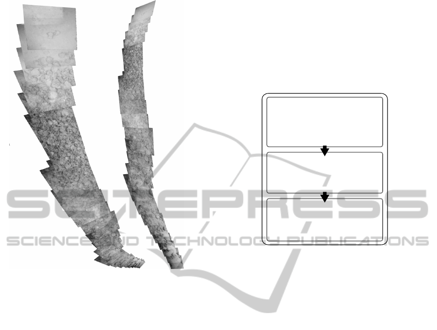
Figure 1: A distorted mosaic due to a wrong reference ho-

mography selection (left). Note that in the former case more

than half of the frames accumulate on the bottom with large

scale variations and distortions. This is not present in the

output given by the proposed method (right). In both cases

no post-processing color correction or blending have been

applied.

Sect. 3, showing the good performance of the overall

algorithm. Finally, conclusions and future work are

draw out in Sect. 4.

2 METHOD DESCRIPTION

2.1 Overview

The overall pipeline of the method is schematically

described in Fig. 2. The approach starts by dividing

the video sequence into successive piecewise planar

sub-mosaics with low geometric distortions with re-

spect to the original image frames, as described in

Sect. 2.2.

Sequential concatenation of temporally consecu-

tive frames is sufﬁcient to produce the piecewise pla-

nar sub-mosaics. However, a global strategy is re-

quired to match frames locally close but temporally

non-consecutive. This is required in order to reduce

the propagation of homography estimation errors due

to the non-planar real nature of the scene.

An approximated 2D map of the video frame po-

sitions is then computed, by considering the average

translation between successive frames, which is up-

dated when two close frames are discovered. The

best paths on the map are used to robustly track fea-

tures in spatially close but non-consecutive frames

and compute the homography between them. De-

tails of this step are given in Sect. 2.3. Finally, as

Sub-mosaic generation:

- consecutive image matching and

homography computation

- sequential greedy homography

concatenation

Feature track map building:

- frame location map generation

- best path computation

- keypoint track across sub-mosaics

Hierachical sub-mosaic merging

- sub-mosaic alignment

- reference homography estimation

- post-processing

Figure 2: A schematic view of the mosaic pipeline.

described in Sect. 2.4, sub-mosaics are merged us-

ing the tracked keypoints one at a time according to

a hierarchical clustering, preferring sub-mosaics with

high overlap. When two sub-mosaics are merged, the

best reference homography between them is found in

order to minimize the distortion of the image frames.

This is achieved by exploring the search space of the

“average” homographies between the two sub-mosaic

images. Common blending and photometric post-

processing steps are eventually applied to reﬁne the

results (Uyttendaele et al., 2001; Kwatra et al., 2003;

Brown and Lowe, 2007; Prados et al., 2012).

2.2 Sub-mosaic Generation

Given the video sequence of n +1 consecutive frames

, I

, . . . , I

, the ﬁrst step is to extract the image

keypoints to obtain the matches between overlapping

frames and their associated homography. For this pur-

pose, the HarrisZ detector (Bellavia et al., 2011) is

used, providing robust and reliable corner features.

In the following step, homographies between con-

secutive image frame pairs (I

, I

k+1

) are computed.

In particular, feature matches are computed using

the sGOr matching selection strategy (Bellavia et al.,

2014) under the further assumption that the optical

ﬂow between successive frames is bounded. That is,

given a generic keypoint pair (x

, x

k+1

) with x

∈ I

, it

must hold

k x

− x

k+1

k< ε

(1)

EstimatingtheBestReferenceHomographyforPlanarMosaicsFromVideos

513

where the threshold ε

is set to a third of the diago-

nal of the rectangular video frame. The homography

k,k+1

∈ R

3×3

that maps points from I

to I

is com-

puted on the obtained matches using the noRANSAC

method (Bellavia and Tegolo, 2011), a robust exten-

sion of the RANSAC 7-point algorithm (Hartley and

Zisserman, 2003) using normalized errors.

Finally, a piecewise planar sub-mosaic S

i, j

going

from frame i to frame j (see Fig. 3) is constructed

from its keyframe sequence K

i, j

= I

, I

, . . . ,I

(2)

with i = k

< k

< . . . < k

= j, as explained here-

after. The ﬁrst image frame and keyframe I

of the

subsequence is used as reference, so that the ho-

mography map H

i, j

relating the sub-mosaic to any

keyframe I

, is simply obtained by concatenating the

sequential homographies from H

i,i+1

to H

w−1

i, j

= H

w−1

w−2

. . . H

i,i+1

(3)

The sub-mosaic is then built according to a greedy

strategy by sequentially looking for next keyframe in

i+1

, I

i+2

, . . .. The frame I

is added as keyframe if the

overlap between the current sub-mosaic and the pro-

jection of frame I

onto the sub-mosaic is less than a

threshold. The sub-mosaic generation process stops

when the projection of frame I

j+1

is too distorted to

be included in K

i j

. In this case I

is added as the ﬁ-

nal keyframe with the sub-mosaic S

i, j

as output and

starting from I

j+1

a new sub-mosaic is grown.

The distortion criterion is deﬁned as follows. As-

suming rectangular video frames, their projections

into quadrilaterals in the mosaic are considered dis-

torted if one of the following conditions is met: (1) the

ratio between the original and projected frames is out-

side a user-deﬁned range, (2) the area of the bounding

box including all common keypoints in the projected

mosaic is below a threshold, (3) the ratio between the

minimum and maximum semi-axis lengths of the pro-

jected quadrilateral exceeds a given value.

2.3 Feature Track Map Building

Sequential sub-mosaics can be merged using only the

homography between boundary keyframes, for exam-

ple using the homography H

j, j+1

between the sub-

mosaics S

i, j

and S

j+1,w

, with i < j < w. However,

this solution is not robust, due to inevitable inaccura-

cies in the homography which may propagate across

the sequence, especially when coming back to an al-

ready seen location of the mosaic. According to this

observation, adding more robust matches and recog-

nizing loop-closures (Konolige and Agrawal, 2008)

may improve the result thanks to a suitable keypoint

tracking strategy, implemented as follows.

Figure 3: From left to right, two consecutive sub-mosaics

from the mosaic of Fig. 1(right). The reference image

frames I

on which successive frames are concatenated (see

text) are highlighted by boxes. No color correction or blend-

ing have been applied.

Given a threshold ε

= 1.5 px the enriched set of

matches M

k−1,k

is computed, considering all the key-

point matching pairs and not only the ﬁltered subset

given in input to the RANSAC (see Sect. 2.2). With

an abuse of notation for indicating homogeneous nor-

malized coordinates, we have

k−1,k

= {(x

k−1

, x

) : x

k−1

∈ I

k−1

∈ I

, k x

− H

k−1,k

k−1

k< ε

}

(4)

where matches are selected according to the nearest

neighbour approach (Lowe, 2004) on the homogra-

phy reprojection error. This allows to track more

keypoints across non-consecutive frames since longer

tracks can be built.

In order to handle loop-closure, a robust global

keypoint tracking map is also implemented, see

Fig. 4. Under the assumption of an almost planar sur-

face, an initial frame location map T

: {I

} → R

for

each frame I

in the video sequence is computed us-

ing the average displacement between corresponding

matches

) = T

k−1

) +

∑

k−1,k

− x

k−1

) (5)

The process is started from T

) = 0, where the

summation is on the match pairs (x

k−1

, x

) ∈ M

k−1,k

and N = |M

k−1,k

| (blue line on Fig. 4(a)). Further it-

erations i are introduced to progressively update the

map T

, as in the case of the Self-Organizing Map

learning method (Haykin, 1998). In detail, given the

VISAPP2015-InternationalConferenceonComputerVisionTheoryandApplications

514

(a) (b)

Figure 4: The frame location map (a) corresponding to the

mosaic in (b). The ﬁrst and last iterations T

and T are

plotted as blue and red lines, respectively, and no blending

and color correction have been applied to the mosaic. The

zoomed region in (a) shows the minimum path A

a,b

and the

best path B

a,b

between two frames I

and I

. The maximum

allowable edge distance is ε

. (Best viewed in color.)

set of frames I

in a radius ε

from I

= {I

: k T

) − T

) k≤ ε

} (6)

where ε

is set as for Eq. 1, T

is updated to T

i+1

follows

i+1

) = T

) +

∑

k,w

∑

k,w

− x

) (7)

where the outer summation is on the frames I

∈ J

L = |J

|, the inner summation as for Eq. 5 and M

k,w

is deﬁned analogously to M

k−1,k

(see Eq. 4). The

value 0 < d < 1 is an exponential decay going with

the iteration i to limit the iterations and g

k,w

is a

Gaussian weight on the distance k T

) − T

) k.

When d

' 0 no further updates are needed, and the

ﬁnal map T is obtained (from blue to red lines as it-

erations proceed in Fig. 4(a)). Note that the planar

displacement approximation of the map cannot han-

dle scale variations, so that there is no perfect cor-

respondence between Fig. 4(a) and Fig. 4(b). Nev-

ertheless, this does not interfere with the ﬁnal key-

point tracking. The graph G = (V, E) is associated

to the map T , where the set of nodes is V = {I

i.e. the frames of the sequence, and an edge E

k,z

be-

tween vertexes I

and I

with an associated weight

k T (I

) − T (I

) k exists only if ∃ i such that I

∈ J

A keypoint x

on frame I

is tracked to the key-

point x

in the frame I

following the chain of matches

, x

), (x

, x

), . . . , (x

, x

) according to the best

path B between the frame I

and I

on the graph G.

For any match pair in the chain it must hold that

, x

) ∈ M

. The best path E

w,k

, E

, . . . E

must concatenates short weight edges, since matches

from distant frames are more unstable and error

prone. Furthermore, the best path length must be

short because very long paths accumulate errors.

We computed the best path B from a frame I

to a frame I

by an extended version of the Floyd-

Warshall all-shortest-paths algorithm (Cormen et al.,

2009). Hereafter, both a path and its length with be

referred with the same symbol. In the ﬁrst step we

compute the minimum path length A between all the

frames in G, using the standard algorithm updating

rule at each iteration 0 ≤ i ≤ |V |, i.e.

a,b

(

i−1

a,c

+ A

i−1

c,b

if A

i−1

a,c

+ A

i−1

c,b

< A

i−1

a,b

i−1

a,b

otherwise

(8)

where A

a,b

is the shortest path length at iteration i be-

tween frames I

and I

, and A

a,b

= E

a,b

. Denoting the

shortest path length at the last iteration by A

a,b

= A

|V |

a,b

this is used as follows to bound the length of the best

path B

a,b

using a factor f = 2. Deﬁning the auxiliary

values C

a,b

representing the maximum edge weight in

the path between I

and I

, the update rule for the last

step are

a,b











i−1

a,c

+ B

i−1

c,b

if B

i−1

a,c

+ B

i−1

c,b

< f A

a,b

and

max(C

i−1

a,c

i−1

c,b

) < C

i−1

a,b

i−1

a,b

otherwise

(9)

and

a,b











max(C

i−1

a,c

i−1

c,b

) if B

i−1

a,c

+ B

i−1

c,b

< f A

a,b

and

max(C

i−1

a,c

i−1

c,b

) < C

i−1

a,b

i−1

a,b

otherwise

(10)

initialized as for the previous step as B

a,b

= C

a,b

, the edge in the best path are updated accordingly.

An example of the best path between two frames is

given in Fig. 4(a).

Denoting the best path at the last iteration with

a,b

= B

|V |

a,b

, referring to Sect. 2.2, the robust matches

between two sub-mosaics S

i, j

and S

w,z

are obtained

by trying to track on the best path B

s,t

each of the

keypoints x

i, j

of any keyframe I

∈ K

i, j

to a keypoint

z,w

of any keyframe I

∈ K

w,z

. The obtained robust

matches M

z,w

i, j

= {(x

i, j

, x

z,w

)} across the sub-mosaics

are used to compute the homography H

z,w

i, j

and ﬁnally

merge the sub-mosaics as explained in the next sec-

tion.

EstimatingtheBestReferenceHomographyforPlanarMosaicsFromVideos

515

Note that for computing the RANSAC given in-

lier set M

z,w

i, j

an error threshold 5 times greater than

that used in the other RANSAC inlier set M

k,w

is em-

ployed. This is done to partially relax the planar sur-

face assumption, which is unreal in concrete cases,

and allow larger surface deformations.

2.4 Hierarchical Sub-mosaic Merging

Sub-mosaics are merged incrementally according to

their overlap, following a hierarchical clustering al-

gorithm. In particular, deﬁning by S

= {S

i, j

} the

initial cluster partition, at each step 0 ≤ i < |S

|, we

try to merge all the possible pairs (S

i, j

, S

w,z

), with

i, j

, S

w,z

∈ S

, using the robust homography H

z,w

i, j

com-

puted as in Sect. 2.3, to which the reference homog-

raphy

z,w

i, j

described next is applied. Denoting by S

∗

i, j

the area of the sub-mosaic S

i, j

according to the ref-

erence homography

z,w

i, j

and in similar way for S

∗

w,z

only the sub-mosaic pair with the minimal overlap er-

ror R

w,z

i, j

w,z

i, j

= 1 −

∗

i, j

∩ S

∗

w,z

∗

i, j

∪ S

∗

w,z

(11)

is effectively merged in the next cluster partition S

i+1

until no more merges can be done. The reference ho-

mography

z,w

i, j

between two sub-mosaics is computed

by trying to minimize the distortion of all the frames

in K

i, j

and K

w,z

in the merged mosaic. In particular,

considering the pair (S

i, j

, S

w,z

), we deﬁne the auxil-

iary merged mosaics S

and S

obtained respectively

using the ﬁrst frames I

∈ K

i, j

and I

∈ K

w,z

as ref-

erences (see Fig. 5 (top and middle rows)). In the

ﬁrst case the homography H

z,w

i, j

is used to map points

of S

z,w

onto the reference frame I

, while in the other

case the inverse (H

z,w

i, j

)

−1

maps points of S

i, j

onto I

Both S

and S

are aligned according to the robust

matches (x

i, j

, x

z,w

) ∈ M

z,w

i, j

(see Sect. 2.3). In partic-

ular, S

and S

are translated so that the new origins

are in their centroids and rotated according to the ro-

tation R of the best similarity transform obtained by

the least-square solution (Zhang and Liu, 2014), i.e.

= x

−

∑

w,z

i, j

(12)

= C





−

∑

w,z

i, j

w,z





(13)

C =

+ b



a b

b a



(14)

where

and

are the aligned new point coordinates

for points x

∈ S

and x

∈ S

respectively. The values

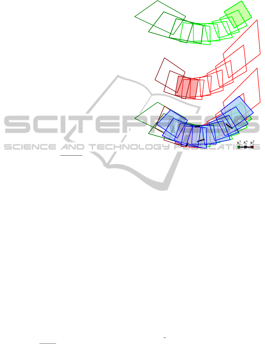
Figure 5: The auxiliary mosaics S

(green frames, top row)

and S

(red frames, middle row) obtained using respec-

tively as reference frames I

∈ K

i, j

(green ﬁlled frame) and

∈ K

w,z

(red ﬁlled frame) from S

i, j

(lighter color) and

w,z

(darker color) are aligned to ﬁnd the best reference ho-

mography (bottom row). Four pairs of corresponding ran-

dom sampled points (x

, x

) are used to generate the mid-

points x

on which computing the reference homography

z,w

i, j

(bottom row, blue frames). The error P is given by

accounting for the distortion of each resulting (blue) frame.

(Best viewed in color).

a and b are computed on lest-squares according to the

similarity transform

i, j





a b c

b a c

0 0 1





w,z

(15)

with an abuse of notation for homogeneous coordi-

nates and a, b, c

, c

∈ R (see Fig. 5 (bottom row,

green and red frames) for an example).

The reference homography

z,w

i, j

is chosen by

RANSAC, looking for the “average” homography

which minimizes the error P (see Fig. 5 (bottom row,

blue frames)). Given four corresponding randomly

sampled non-collinear points x

and x

on S

and

respectively, 1 ≤ i ≤ 4, and the associated mid-

points x

+ x

), the “average” homography is

given by the homography H

mapping x

to x

. Un-

der the assumption of n × m rectangular frames, for

each frame I

∈ K

i, j

∪ K

w,z

, we compute a distortion

error P on the quadrilateral

, obtained by applying

VISAPP2015-InternationalConferenceonComputerVisionTheoryandApplications

516

to the image of I

on S

P = max

∈K

i, j

∪K

w,z

+ P

) (16)

Figure 6: Conﬁguration for computing the error P when

projecting the image frame I

through the mosaic ho-

mography H (see text). Corresponding vertex pairs are

) for 1 ≤ i ≤ 4.

Considering the four quadrilateral sides of length

in consecutive order, under the assumption that

n > m with l

, l

corresponding to the side of length

n on I

and in similar way l

, l

to m (see Fig. 6), we

deﬁne the different errors composing P. In particular,

measures the error on the ratio between the oppo-

site sides of

= 2 −



min(l

, l

)

max(l

, l

)

min(l

, l

)

max(l

, l

)



(17)

while P

measures the error on the ratio between con-

secutive sides of

= 1 −

min(r,

)

max(r,

)

(18)

where

r = min





(19)

The error P

gives the error ratio between the frame

area nm and the area of its image A

= 1 −

min(A

, nm)

max(A

, nm)

(20)

while P

measures the angular error

= (max(cos

, cos

))

(21)

cos

being the absolute value of the cosine between

the two sides l

and l

. An example of resulting mo-

saic obtained by merging sub-mosaics according to

the best reference homography

z,w

i, j

of Fig. 5 is shown

in Fig. 7. Finally, as post-processing step on the ﬁ-

nal merged mosaic, multi-band blending (Brown and

Lowe, 2007) and color correction using an extension

of the Reinhard’s method (Reinhard et al., 2001) are

applied.

Figure 7: The initial sub-mosaics S

i, j

, S

w,z

(top) and the re-

sulting mosaic (bottom) according to the computed refer-

ence homography

z,w

i, j

of Fig. 5. In both cases no post-

processing color correction or blending have been applied.

(a) (b)

Figure 8: Snapshots of the two test video sequences. In the

case the video sequence (a) the shaded area containing a

ﬁxed robot arm has been cropped. (Best viewed in color.)

3 EXPERIMENTAL RESULTS

We tested the proposed pipeline on two underwa-

ter video sequences which together with the software

code are freely available online

. Snapshots of video

frames are shown in Fig. 8, in the case of the ﬁrst

video, the image area of the frame including the robot

arm was cropped. To remove redundant data, the orig-

inal 25 fps videos were downsampled to 5 fps. The

corresponding output mosaics are shown in Fig. 9.

As it can be noted, the resulting mosaics are good,

with no evident misalignment glitches or strong frame

deformations. Underwater scenes are very challeng-

ing, due to their high intensity changes and repeated

patterns, which make the feature tracking difﬁcult, so

http://www.math.unipa.it/fbellavia/dl/mosaic.zip

EstimatingtheBestReferenceHomographyforPlanarMosaicsFromVideos

517

(a) (b)

Figure 9: Output mosaics corresponding respectively to the video sequences of Fig. 8(a)-(b). (Best viewed in color).

VISAPP2015-InternationalConferenceonComputerVisionTheoryandApplications

518

that the quality of the results strengthen the validity of

the feature track map computation of Sect. 2.3.

As it can be seen from the output mosaics, the pro-

posed method is effective in choosing the reference

mosaic homography (see Sect. 2.4). Note that, us-

ing the ﬁrst image frame as reference, in the case of

Fig. 8(a) would lead to very distorted images, as can

be observed even from corresponding initial merged

sub-mosaics (see Fig. 5 (top and middle rows, green

and red frames)). Indeed, the proposed method al-

lowed us to get in a completely automatic way as

good-looking mosaics as those obtained with strong

expert user intervention.

4 CONCLUSIONS

This paper proposes a new approach to compute the

best reference mosaic homography that minimizes the

frame distortions in the case of planar mosaics. For

this purpose, a full hierarchical mosaicing pipeline

was designed, with particular attention to underwa-

ter mosaicing applications that, due to the scene com-

plexity, require robust feature tracking schemes as the

one proposed in this paper. Experimental results show

the validity of our method, yielding to high quality

unsupervised mosaics.

Future work will include more evaluation tests as

well incorporating in the pipeline new stitching algo-

rithms (Zaragoza et al., 2014; Zhang and Liu, 2014)

to replace the standard 7-point homography compu-

tation, with the aim to improve results in the case of

strong 3D content.

ACKNOWLEDGEMENT

Thanks to Pamela Gambogi of the “Soprintendenza

per i Beni Archeologici della Toscana”, Italian Min-

istry of Culture, for providing the input video se-

quences.

This work has been carried out during the AR-

ROWS project, supported by the European Commis-

sion under the Environment Theme of the “7th Frame-

work Programme for Research and Technological De-

velopment”.

REFERENCES

Bellavia, F., Gagliano, G., Tegolo, D., and Valenti, C.

(2007). Global archaeological mosaicing for under-

water scenes. WSEAS Transactions on Signal Process-

ing, 2(7):997–1003.

Bellavia, F. and Tegolo, D. (2011). noRANSAC for funda-

mental matrix estimation. In British Machine Vision

Conference, pages 1–11.

Bellavia, F., Tegolo, D., and Valenti, C. (2011). Improving

Harris corner selection strategy. IET Computer Vision,

5(2):87–96.

Bellavia, F., Tegolo, D., and Valenti, C. (2014). Keypoint

descriptor matching with context-based orientation es-

timation. Image and Vision Computing, 32(9):559 –

567.

Brown, M. and Lowe, D. G. (2007). Automatic panoramic

image stitching using invariant features. International

Journal of Computer Vision, 74(1):59–73.

Capel, D. P. (2001). Image Mosaicing and Super-resolution.

PhD thesis, University of Oxford.

Cormen, T. H., Leiserson, C. E., Rivest, R. L., and Stein,

C. (2009). Introduction to Algorithms (3. ed.). MIT

Press.

Hartley, R. and Zisserman, A. (2003). Multiple View Geom-

etry in Computer Vision. Cambridge University Press,

2 edition.

Haykin, S. (1998). Neural Networks: A Comprehensive

Foundation. Prentice Hall, 2 edition.

Konolige, K. and Agrawal, M. (2008). Frameslam: From

bundle adjustment to real-time visual mapping. IEEE

Transactions on Robotics, 24(5):1066–1077.

Kwatra, V., Sch

odl, A., Essa, I. A., Turk, G., and Bobick,

A. F. (2003). Graphcut textures: image and video syn-

thesis using graph cuts. 22(3):277–286.

Lin, W. Y., Liu, S., Matsushita, Y., Ng, T. T., and Cheong,

L. F. (2011). Smoothly varying afﬁne stitching. In

IEEE Conference on Computer Vision and Pattern

Recognition, pages 345–352.

Lowe, D. G. (2004). Distinctive image features from scale-

invariant keypoints. International Journal of Com-

puter Vision, 60(2):91–110.

Pizarro, O. and Singh, H. (2003). Toward large-area mo-

saicing for underwater scientiﬁc applications. IEEE

Journal of Oceanic Engineering, 28(4):651–672.

Prados, R., Garcia, R., Gracias, N., Escartin, J., and Neu-

mann, L. (2012). A novel blending technique for un-

derwater giga-mosaicing. IEEE Journal of Oceanic

Engineering, 37(4):626–644.

Reinhard, E., Ashikhmin, M., Gooch, B., and Shirley, P.

(2001). Color transfer between images. IEEE Com-

puter Graphics and Applications, 21(5):34–41.

Uyttendaele, M., Eden, A., and Szeliski, R. (2001). Elim-

inating ghosting and exposure artifacts in image mo-

saics. In Computer Vision and Pattern Recognition,

pages 509–516.

Zaragoza, J., Chin, T. J., Tran, Q. H., Brown, M., and Suter,

D. (2014). As-Projective-As-Possible image stitching

with moving DLT. IEEE Transaction on Pattern Anal-

ysis and Machine Intelligence, 36(7):1285–1298.

Zhang, F. and Liu, F. (2014). Parallax-tolerant image stitch-

ing. In IEEE Conference on Computer Vision and Pat-

tern Recognition, pages 3262–3269.

EstimatingtheBestReferenceHomographyforPlanarMosaicsFromVideos

519