
CURFIL: Random Forests for Image Labeling on GPU
Hannes Schulz, Benedikt Waldvogel, Rasha Sheikh and Sven Behnke
University of Bonn, Computer Science Institute VI, Autonomous Intelligent Systems,
Friedrich-Ebert-Allee 144, 53113 Bonn, Germany
Keywords:
Random Forest, Computer Vision, Image Labeling, GPU, CUDA.
Abstract:
Random forests are popular classifiers for computer vision tasks such as image labeling or object detection.
Learning random forests on large datasets, however, is computationally demanding. Slow learning impedes
model selection and scientific research on image features. We present an open-source implementation that
significantly accelerates both random forest learning and prediction for image labeling of RGB-D and RGB
images on GPU when compared to an optimized multi-core CPU implementation. We use the fast training
to conduct hyper-parameter searches, which significantly improves on previous results on the NYU depth v2
dataset. Our prediction runs in real time at VGA resolution on a mobile GPU and has been used as data term in
multiple applications.
1 INTRODUCTION
Random forests are ensemble classifiers that are popu-
lar in the computer vision community. Random deci-
sion trees are used when the hypothesis space at every
node is huge, so that only a random subset can be ex-
plored during learning. This restriction is countered
by constructing an ensemble of independently learned
trees—the random forest.
Variants of random forests were used in computer
vision to improve e.g. object detection or image seg-
mentation. One of the most prominent examples is
the work of (Shotton et al., 2011), who use random
forests in Microsoft’s Kinect system for the estimation
of human pose from single depth images. Here, we are
interested in the more general task of image labeling,
i.e. determining a label for every pixel in an
RGB
or
RGB-D image (Fig. 1).
The real-time applications such as the ones pre-
sented by (Lepetit et al., 2005) and (Shotton et al.,
2011) require fast prediction in few milliseconds per
image. This is possible with parallel architectures such
as
GPU
s, since every pixel can be processed indepen-
dently. Random forest training for image labeling,
however, is not as regular—it is a time consuming pro-
cess. To evaluate a randomly generated feature candi-
date in a single node of a single tree, a potentially large
number of images must be accessed. With increasing
depth, the number of pixels in an image arriving in the
current node can be very small. It is therefore essential
for the practitioner to optimize memory efficiency in
Figure 1: Overview of image labeling with random forests:
Every pixel (
RGB
and depth) is classified independently
based on its context by the trees of a random forest. The leaf
distributions of the trees determine the predicted label.
various regimes, or to resort to large clusters for the
computation. Furthermore, changing the visual fea-
tures and other hyper-parameters requires a re-training
of the random forest, which is costly and impedes
efficient scientific research.
This work describes the architecture of our open-
source
GPU
implementation of random forests for im-
age labeling (
CURFIL
). C
URFIL
provides optimized
CPU
and
GPU
implementations for the training and
prediction of random forests. Our library trains ran-
dom forests up to 26 times faster on
GPU
than our
optimized multi-core
CPU
implementation. Prediction
is possible in real-time speed on a single mobile GPU.
In short, our contributions are as follows:
1. we describe how to efficiently implement random
forests for image labeling on GPU,
2.
we describe a method which allows to train on
156
Schulz H., Waldvogel B., Sheikh R. and Behnke S..
CURFIL: Random Forests for Image Labeling on GPU.
DOI: 10.5220/0005316201560164
In Proceedings of the 10th International Conference on Computer Vision Theory and Applications (VISAPP-2015), pages 156-164
ISBN: 978-989-758-090-1
Copyright
c
2015 SCITEPRESS (Science and Technology Publications, Lda.)

horizontally flipped images at significantly reduced
cost,
3.
we show that our
GPU
implementation is up to
26 times faster for training (up to 48 times for
prediction) than an optimized multi-core
CPU
im-
plementation,
4.
we show that simply by the now feasible optimiza-
tion of hyper-parameters, we can improve perfor-
mance in two image labeling tasks, and
5.
we make our documented, unit-tested, and
MIT
-
licensed source code publicly available
1
.
The remainder of this paper is organized as follows.
After discussing related work, we introduce random
forests and our node tests in Sections 3 and 4, respec-
tively. We describe our optimizations in Section 5.
Section 6 analyzes speed and accuracy attained with
our implementation.
2 RELATED WORK
Random forests were popularized in computer vision
by (Lepetit et al., 2005). Their task was to classify
patches at pre-selected keypoint locations, not—as in
this work—all pixels in an image. Random forests
proved to be very efficient predictors, while training
efficiency was not discussed. Later work focused on
improving the technique and applying it to novel tasks.
(Lepetit and Fua, 2006) use random forests to clas-
sify keypoints for object detection and pose estimation.
They evaluate various node tests and show that while
training is increasingly costly, prediction can be very
fast.
The first
GPU
implementation for our task was pre-
sented by (Sharp, 2008), who implements random
forest training and prediction for Microsoft’s Kinect
system that achieves a prediction speed-up of 100 and
training speed-up factor of eight on a
GPU
, compared
to a
CPU
. This implementation is not publicly avail-
able and uses
D
irect
3D
which is only supported on the
Microsoft Windows platform.
An important real-world application of image la-
beling with random forests is presented by (Shotton
et al., 2011). Human pose estimation is formulated
as a problem of determining pixel labels correspond-
ing to body parts. The authors use a distributed
CPU
implementation to reduce the training time, which is
nevertheless one day for training three trees from one
million synthetic images on a 1,000
CPU
core cluster.
Their implementation is also not publicly available.
Several fast implementations for general-purpose
random forests are available, notably in the scikit-learn
1
https://github.com/deeplearningais/curfil/
machine learning library (
?
) for
CPU
and CudaTree
(Liao et al., 2013) for
GPU
. General random forests
cannot make use of texture caches optimized for im-
ages though, i.e., they treat all samples separately. G
PU
implementations of general-purpose random forests
also exist, but due to the irregular access patterns
when compared to image labeling problems, their so-
lutions were found to be inferior to
CPU
(Slat and
Lapajne, 2010) or focused on prediction (Van Essen
et al., 2012).
The prediction speed and accuracy of random
forests facilitates applications interfacing computer vi-
sion with robotics, such as semantic prediction in com-
bination with self localization and mapping (St
¨
uckler
et al., 2012) or 6D pose estimation (Rodrigues et al.,
2012) for bin picking.
C
URFIL
was successfully used by (St
¨
uckler et al.,
2013) to predict and accumulate semantic classes of
indoor sequences in real-time, and by (M
¨
uller and
Behnke, 2014) to significantly improve image labeling
accuracy on a benchmark dataset.
3 RANDOM FORESTS
Random forests—also known as random decision trees
or random decision forests—were independently in-
troduced by (Ho, 1995) and (Amit and Geman, 1997).
(Breiman, 2001) coined the term “random forest”.
Random decision forests are ensemble classifiers that
consist of multiple decision trees—simple, commonly
used models in data mining and machine learning. A
decision tree consists of a hierarchy of questions that
are used to map a multi-dimensional input value to an
output which can be either a real value (regression) or
a class label (classification). Our implementation fo-
cuses on classification but can be extended to support
regression.
To classify input
x
, we traverse each of the
K
de-
cision trees
T
k
of the random forest
F
, starting at the
root node. Each inner node defines a test with a binary
outcome (i.e. true or false). We traverse to the left
child if the test is positive and continue with the right
child otherwise. Classification is finished when a leaf
node
l
k
(x)
is reached, where either a single class label
or a distribution
p(c|l
k
(x))
over class labels
c ∈ C
is
stored.
The
K
decision trees in a random forest are trained
independently. The class distributions for the input
x
are collected from all leaves reached in the decision
trees and combined to generate a single classification.
Various combination functions are possible. We imple-
ment majority voting and the average of all probability
CURFIL:RandomForestsforImageLabelingonGPU
157

q
w
1
w
2
h
1
h
2
o
1
o
2
Figure 2: Sample visual feature at three different query
pixels. Feature response is calculated from difference of
average values in two offset regions. Relative offset locations
o
i
and region extents
w
i
,
h
i
are normalized with the depth
d(q) at the query pixel q.
distributions as defined by
p(c|F ,x) =
1
K
K
∑
k=1
p(c|l
k
(x)).
Key difference between a decision tree and a ran-
dom decision tree is the training phase. The idea of
random forests is to train multiple trees on different
random subsets of the dataset and random subsets of
features. In contrast to normal decision trees, random
decision trees are not pruned after training, as they
are less likely to overfit (Breiman, 2001). Breiman’s
random forests use
CART
as tree growing algorithm
and are restricted to binary trees for simplicity. The
best split criterion in a decision node is selected ac-
cording to a score function measuring the separation
of training examples. C
URFIL
supports information
gain and normalized information gain (Wehenkel and
Pavella, 1991) as score functions.
A special case of random forests are random ferns,
which use the same feature in all nodes of a hierarchy
level. While our library also supports ferns, we do not
discuss them further in this paper, as they are neither
faster to train nor did they produce superior results.
4 VISUAL FEATURES FOR NODE
TESTS
Our selection of features was inspired by (Lepetit et al.,
2005)—the method for visual object detection pro-
posed by (Viola and Jones, 2001). We implement
two types of
RGB-D
image features as introduced by
(St
¨
uckler et al., 2012). They resemble the features of
(Sharp, 2008; Shotton et al., 2011)—but use depth-
normalization and region averages instead of single
pixel values. (Shotton et al., 2011) avoid the use of
Algorithm 1: Training of random decision tree.
Require: D training instances
Require: F
number of feature candidates to generate
Require: P number of feature parameters
Require: T number of thresholds to generate
Require: stopping criterion (e.g. maximal depth)
1: D ← randomly sampled subset of D (D ⊂ D)
2: N
root
← create root node
3: C ←
{
(N
root
,D)
}
initialize candidate nodes
4: while C 6=
/
0 do
5: C
0
←
/
0
initialize new set of candidate nodes
6: for all (N, D) ∈ C do
7:
D
left
,D
right
← EVAL BESTSPLIT(D)
8: if ¬STOP(N, D
left
) then
9: N
left
← create left child for node N
10: C
0
← C
0
∪
{
(N
left
,D
left
)
}
11: if ¬STOP(N, D
right
) then
12: N
right
← create right child for node N
13: C
0
← C
0
∪
N
right
,D
right
14: C ← C
0
continue with new set of nodes
region averages to keep computational complexity low.
For
RGB
-only datasets, we employ the same features
but assume constant depth. The features are visualized
in Fig. 2.
For a given query pixel
q
, the image feature
f
θ
is
calculated as the difference of the average value of the
image channel
φ
i
in two rectangular regions
R
1
,R
2
in
the neighborhood of
q
. Size
w
i
,h
i
and 2D offset
o
i
of
the regions are normalized by the depth d(q):
f
θ
(q) :=
1
|R
1
(q)|
∑
p∈R
1
φ
1
(p) −
1
|R
2
(q)|
∑
p∈R
2
φ
2
(p)
R
i
(q) :=
q +
o
i
d(q)
,
w
i
d(q)
,
h
i
d(q)
. (1)
C
URFIL
optionally fills in missing depth measure-
ments. We use integral images to efficiently com-
pute region sums. The large space of eleven fea-
ture parameters—region sizes, offsets, channels, and
thresholds—requires to calculate feature responses on-
the-fly since pre-computing all possible values in ad-
vance is not feasible.
5 CURFIL SOFTWARE PACKAGE
C
URFIL
’s speed is the result of careful optimization of
GPU
memory throughput. This is a non-linear process
to find fast combinations of memory layouts, algo-
rithms and exploitable hardware capabilities. In the
following, we describe the most relevant aspects of
our implementation.
VISAPP2015-InternationalConferenceonComputerVisionTheoryandApplications
158

Block (0, D) Block (1, D) Block (2, D)
Block (0, 1) Block (1, 1) Block (2, 1)
Block (X, D)
Block (X, 1)
Block (0, 0) Block (1, 0) Block (2, 0) Block (X, 0)
…
scheduling order
Feature
Sample
(a) Feature Response Kernel
Block (0, F) Block (1, F) Block (2, F)
Block (0, 1) Block (1, 1) Block (2, 1)
Block (T, F)
Block (T, 1)
Block (0, 0) Block (1, 0) Block (2, 0) Block (T, 0)
…
scheduling order
Threshold
Feature
Thread Block (2,0)
Thread 0 Thread 1 Thread 2 Thread 3 Thread X
…
(b) Histogram Aggegation Kernel
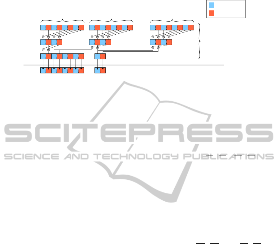
Figure 3:
(a)
Two-dimensional grid layout of the feature response kernel for
D
samples and
F
features. Each block contains
n
threads. The number of blocks in a row,
X
, depends on the number of features.
X =
d
F
/n
e
. Feature responses for a given
sample are calculated by the threads in one block row. The arrow (red dashes) indicates the scheduling order of blocks.
(b)
Thread block layout of the histogram aggregation kernel for
F
features and
T
thresholds. One thread block per feature and per
threshold.
X
threads in block aggregate histogram counters for
D
samples in parallel. Every thread iterates over at most
d
D
/X
e
samples.
User API.
The
CURFIL
software package includes
command line tools as well as a library for random
forest training and prediction. Inputs consist of images
for
RGB
, depth, and label information. Outputs are
forests in
JSON
format for training and label-images
for prediction. Datasets with varying aspect ratios are
supported.
Our source code is organized such that it is easy
to improve and change the existing visual feature im-
plementation. It is developed in a test-driven process.
Unit tests cover major parts of our implementation.
CPU Implementation.
Our
CPU
implementation is
based on a refactored, parallelized and heavily opti-
mized version of the Tuwo Computer Vision Library
2
by Nowozin. Our optimizations make better use of
CPU
cache by looping over feature candidates and
thresholds in the innermost loop, and by sorting the
dataset according to image before learning. Since fea-
ture candidate evaluations do not depend on each other,
we can parallelize over the training set and make use
of all
CPU
cores even when training only a single tree.
GPU Implementation.
Evaluation of the optimized
random forest training on
CPU
(Algorithm 1) shows
that the vast majority of time is spent in the evaluation
of the best split feature. This is to our benefit when
accelerating random forest training on
GPU
. We re-
strict the
GPU
implementation efforts to the relatively
short feature evaluation algorithm (Algorithm 2) as a
drop-in replacement and leave the rest of the
CPU
com-
putation unchanged. We use the
CPU
implementation
2
http://www.nowozin.net/sebastian/tuwo/
as a reference for the
GPU
and ensure that results are
the same in both implementations.
Split evaluation can be divided into the following
four phases that are executed in sequential order:
1.
random feature and threshold candidate genera-
tion,
2. feature response calculation,
3.
histogram aggregation for all features and thresh-
old candidates, and
4. impurity score (information gain) calculation.
Each phase depends on results of the previous phase.
As a consequence, we cannot execute two or more
phases in parallel. The
CPU
can prepare data for the
launch of the next phase, though, while the
GPU
is
busy executing the current phase.
Algorithm 2: CPU-optimized feature evaluation.
Require: D samples
Require: F ∈ R
F×P
random feature candidates
Require: T ∈ R
F×T
random threshold candidates
1: initialize histograms for every feature/threshold
2: for all d ∈ D do
3: for all f ∈ 1 ...F do
4: calculate feature response
5: for all θ ∈ T
f
do
6: update according histogram
7: calculate impurity scores for all histograms
8: return histogram with best score
CURFIL:RandomForestsforImageLabelingonGPU
159
class 0
…
0
1 2
3
C
shared
memory
…
global
memory
left counter
right counter
class
thread
0
1 2
3
4
5 6
7
2C
…
…
class 1 class C
…
Figure 4: Reduction of histogram counters. Every thread sums to a dedicated left and right counter (indicated by different
colors) for each class (first row). Counters are reduced in a subsequent phase. The last reduction step stores counters in shared
memory, such that no bank conflicts occur when copying to global memory.
5.1 GPU Kernels
Random Feature and Threshold Candidate Gener-
ation.
A significant amount of training time is used
for generating random feature candidates. The total
time for feature generation increases per tree level
since the number of nodes increases as trees are grown.
The first step in the feature candidate generation
is to randomly select feature parameter values. These
are stored in a
F×11
matrix for
F
feature candidates
and eleven feature parameters of Eq.
(1)
. The sec-
ond step is the selection of one or more thresholds
for every feature candidate. Random threshold can-
didates can either be obtained by randomly sampling
from a distribution or by sampling feature responses of
training instances. We implement the latter approach,
which allows for greater flexibility if features or im-
age channels are changed. For every feature candidate
generation, one thread on the
GPU
is used and all
T
thresholds for a given feature are sampled by the same
thread.
In addition to sorting samples according to the im-
age they belong to, feature candidates are sorted by the
feature type, channels used, and region offsets. Sort-
ing reduces branch divergence and improves spatial
locality, thereby increasing the cache hit rate.
Feature Response Calculation.
The
GPU
imple-
mentation uses a similar optimization technique to
the one used on the
CPU
, where loops in the feature
generation step are rearranged in order to improve
caching.
We used one thread to calculate the feature re-
sponse for a given feature and a given training sample.
Figure 3(a) shows the thread block layout for the fea-
ture response calculation. A row of blocks calculates
all feature responses for a given sample. A column of
blocks calculates the feature responses for a given fea-
ture over all samples. The dotted red arrow indicates
the order of thread block scheduling. The execution
order of thread blocks is determined by calculating
the Block ID
bid
. In the two-dimensional case, it is
defined as
bid = blockIdx.x + gridDim.x
| {z }
blocks in row
·blockIdx.y
| {z }
sample ID
.
The number of features can exceed the maximum num-
ber of threads in a block, hence, the feature response
calculation is split into several thread blocks. We use
the
x
coordinate in the grid for the feature block to
ensure that all features are evaluated before the
GPU
continues with the next sample. The
y
coordinate in the
grid assigns training samples to thread blocks. Threads
reconstruct their feature ID
f
using block size, thread
and block ID by calculating
f = threadIdx.x + blockDim.x
| {z }
threads in block row
· blockIdx.x
| {z }
block index in grid row
.
After sample data and feature parameters are
loaded, the kernel calculates a single feature response
for a depth or color feature by querying four pixels in
an integral image and carrying out simple arithmetic
operations to calculate the two regions sums and their
difference.
Histogram Aggregation.
Feature responses are ag-
gregated into class histograms. Counters for his-
tograms are maintained in a four-dimensional matrix
of size
F×T ×C×2
for
F
features,
T
thresholds,
C
classes, and the two left and right children of a split.
To compute histograms, the iteration over features
and thresholds is implemented as thread blocks in a
two-dimensional grid on
GPU
; one thread block per
feature and threshold. This is depicted in Fig. 3(b).
Each thread block slices samples into partitions such
that all threads in the block can aggregate histogram
counters in parallel.
VISAPP2015-InternationalConferenceonComputerVisionTheoryandApplications
160

Histogram counters for one feature and threshold
are kept in the shared memory, and every thread gets
a distinct region in the memory. For
X
threads and
C
classes,
2XC
counters are allocated. An additional
reduction phase is then required to reduce the counters
to a final sum matrix of size
C×2
for every feature and
threshold.
Figure 4 shows histogram aggregation and sum re-
duction. Every thread increments a dedicated counter
for each class in the first phase. In the next phase, we
iterate over all
C
classes and reduce the counters of
every thread in
O(logX)
steps, where
X
is the number
of threads in a block. In a single step, every thread
calculates the sum of two counters. The loop over all
classes can be executed in parallel by
2C
threads that
copy the left and right counters of C classes.
The binary reduction of counters (Fig. 4) has a
constant runtime overhead per class. The reduction of
counters for classes without samples can be skipped,
as all counters are zero in this case.
Impurity Score Calculation.
Computing impurity
scores from the four-dimensional counter matrix is the
last of the four training phases that are executed on
GPU.
In the score kernel computation, 128 threads per
block are used. A single thread computes the score
for a different pair of features and thresholds. It loads
2C
counters from the four-dimensional counter matrix
in global memory, calculates the impurity score and
writes back the resulting score to global memory.
The calculated scores are stored in a
T ×F
matrix
for
T
thresholds and
F
features. The matrix is then
finally transferred from device to host memory space.
Undefined Values.
Image borders and missing
depth values (e.g. due to material properties or camera
disparity) are represented as NaN, which automatically
propagates and causes comparisons to produce false.
This is advantageous, since no further checks are re-
quired and the random forest automatically learns to
deal with missing values.
5.2 Global Memory Limitations
Slicing of Samples.
Training arbitrarily large
datasets with many samples can exceed the storage
capacity of global memory. The feature response ma-
trix of size
D×F
scales linearly in the number of sam-
ples
D
and the number of feature candidates
F
. We
cannot keep the entire matrix in global memory if
D
or
F
is too large. For example, training a dataset
with 500 images, 2000 samples per image, 2000 fea-
ture candidates and double precision feature responses
(
64 b
it) would require
500·2000 ·2000·64 bit ≈ 15GB
of global memory for the feature response matrix in
the root node split evaluation.
To overcome this limitation, we split samples into
partitions, sequentially compute feature responses, and
aggregate histograms for every partition. The maxi-
mum possible partition size depends on the available
global memory of the GPU.
Image Cache.
Given a large dataset, we might not
be able to keep all images in the
GPU
global memory.
We implement an image cache with a last recently used
(
LRU
) strategy that keeps a fixed number of images in
memory. Slicing samples ensures that a partition does
not require more images than can be fit into the cache.
Memory Pooling.
To avoid frequent memory allo-
cations, we reuse memory that is already allocated but
no longer in use. Due to the structure of random deci-
sion trees, evaluation of the root node split criterion is
guaranteed to require the largest amount of memory,
since child nodes always contain less or equal samples
than the root node. Therefore, all data structures have
at most the size of the structures used for calculating
the root node split. With this knowledge, we are able
to train a tree with no memory reallocation.
5.3 Extensions
Hyper-parameter Optimization.
Cross-validating
all the hyper-parameters is a requirement for model
comparison, and random forests have quite a few
hyper-parameters, such as stopping criteria for split-
ting, number of features and thresholds generated, and
the feature distribution parameters.
To facilitate model comparison,
CURFIL
includes
support for cross-validation and a client for an in-
formed search of the best parameter setting using Hy-
peropt (Bergstra et al., 2011). This allows to leverage
the improved training speed to run many experiments
serially and in parallel.
Image Flipping.
To avoid overfitting, the dataset
can be augmented using transformations of the train-
ing dataset. One possibility is to add horizontally
flipped images, since most tasks are invariant to this
transformation. C
URFIL
supports training horizontally
flipped images with reduced overhead.
Instead of augmenting the dataset with flipped im-
ages and doubling the number of pixels used for train-
ing, we horizontally flip each of the two rectangular
regions used as features for a sampled pixel. This is
equivalent to computing the feature response of the
same feature for the same pixel on an actual flipped
image. Histogram counters are then incremented fol-
lowing the binary test of both feature responses. The
CURFIL:RandomForestsforImageLabelingonGPU
161

Table 1: Comparison of random forest training time (in min-
utes) on a quadcore
CPU
and two non-mobile
GPU
s. Random
forest parameters were chosen for best accuracy.
NYU MSRC
Device time factor time factor
i7–4770K 369 1.0 93.2 1.0
Tesla K20c 55 6.7 5.1 18.4
GTX Titan 24 15.4 3.4 25.9
Table 2: Random forest prediction time in milliseconds, on
RGB-D
images at original resolution, comparing speed on
a recent quadcore
CPU
and various
GPU
s. Random forest
parameters are are chosen for best accuracy.
NYU MSRC-21
Device time factor time factor
i7-440K 477 1 409 1
GTX 675M 28 17 37 11
Tesla K20c 14 34 10 41
GTX Titan 12 39 9 48
implicit assumption here is that the samples generated
through flipping are independent.
The paired sample is propagated down a tree until
the outcome of a node binary test is different for the
two feature responses, indicating that a sample and
its flipped counterpart should split into different direc-
tions. A copy of the sample is then created and added
to the samples list of the other node child.
This technique reduces training time since choos-
ing independent samples from actually flipped images
requires loading more images in memory during the
best split evaluation step. Since our performance is
largely bounded by memory throughput, dependent
sampling allows for higher throughput at no cost in
accuracy.
6 EXPERIMENTAL RESULTS
We evaluate our library on two common image label-
ing tasks, the NYU Depth v2 dataset and the MSRC-21
dataset. We focus on the processing speed, but also
discuss the prediction accuracies attained. Note that
the speed between datasets is not comparable, since
dataset sizes differ and the forest parameters were cho-
sen separately for best accuracy.
The
NYU
Depth v2 dataset by (Silberman et al.,
2012) contains 1,449 densely labeled pairs of aligned
RGB-D
images from 464 indoor scenes. We focus on
the semantic classes ground, furniture, structure, and
props defined by (Silberman et al., 2012).
Table 3: Segmentation accuracies on
NYU
Depth v2 dataset
of our random forest compared to state-of-the-art methods.
We used the same forest as in the training/prediction time
comparisons of Tables 1 and 2.
Accuracy [%]
Method Pixel Class
(Silberman et al., 2012) 59.6 58.6
(Couprie et al., 2013) 63.5 64.5
Our random forest
∗
68.1 65.1
(St
¨
uckler et al., 2013)
∗∗
70.6 66.8
(Hermans et al., 2014) 68.1 69.0
(M
¨
uller and Behnke, 2014)
∗∗
72.3 71.9
∗
see main text for hyper-parameters used
∗∗
based on our random forest prediction.
To evaluate our performance without depth, we use
the
MSRC
-21 dataset
3
. Here, we follow the literature
in treating rarely occuring classes horse and mountain
as void and train/predict the remaining 21 classes on
the standard split of 335 training and 256 test images.
Tables 1 and 2 show random forest training and
prediction times, respectively, on an Intel Core i7-
4770K (
3.9 GHz
) quadcore
CPU
and various
NV
idia
GPUs. Note that the CPU version is using all cores.
For the
RGB-D
dataset, training speed is improved
from
369 min
to
24 min
, which amounts to a speed-up
factor of 15. Dense prediction improves by factor of
39 from 477 ms to 12 ms.
Training on the
RGB
dataset is finished after
3.4 min
on a
GTX
Titan, which is
26
times faster than
CPU
(
93 min
). For prediction, we achieve a speed-up
of 48 on the same device (9 ms vs. 409 ms).
Prediction is fast enough to run in real time even
on a mobile
GPU
(
GTX
675M, on a laptop computer
fitted with a quadcore i7-3610QM
CPU
), with
28 ms
(RGB-D) and 37 ms (RGB).
Our implementation is fast enough to train hun-
dreds of random decision trees per day on a sin-
gle
GPU
. This fast training enabled us to conduct
an extensive parameter search with cross-validation
to optimize segmentation accuracy of a random for-
est trained on the
NYU
Depth v2 dataset (Silberman
et al., 2012). Table 3 shows that we outperform other
state-of-the art methods simply by using a random
forest with optimized parameters. Our implementa-
tion was used in two publications which improved the
results further by 3D accumulation of predictions in
real time (St
¨
uckler et al., 2013) and superpixel
CRF
s
(M
¨
uller and Behnke, 2014)
. This shows that efficient
hyper-parameter search is crucial for model selection.
Example segmentations are displayed in Figs. 5 and 6.
3
http://jamie.shotton.org/work/data.html
VISAPP2015-InternationalConferenceonComputerVisionTheoryandApplications
162
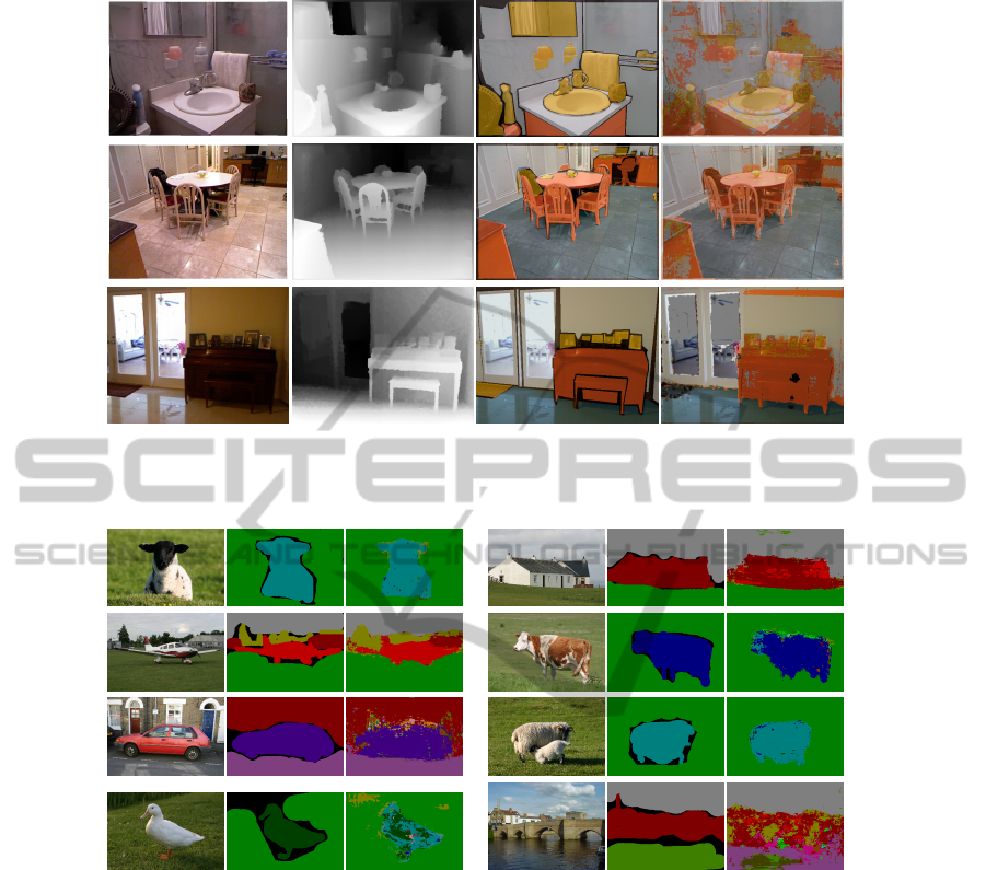
Figure 5: Image labeling examples on
NYU
Depth v2 dataset. Left to right:
RGB
image, depth visualization, ground truth,
random forest segmentation.
Figure 6: Image labeling examples on the
MSRC
-21 dataset. In groups of three: input image, ground truth, random forest
segmentation. Last row shows typical failure cases.
Methods on the established
RGB
-only
MSRC
-21
benchmark are so advanced that their accuracy cannot
simply be improved by a random forest with better
hyper parameters. Our pixel and class accuracies for
MSRC
-21 are
59.2%
and
47.0%
, respectively. This is
still higher than other published work using random
forests as the baseline method, such as
49.7 %
and
34.5 %
by (Shotton et al., 2008). However, as (Shotton
et al., 2008) and the above works show, random forest
predictions are fast and constitute a good initialization
for other methods such as conditional random fields.
Finally, we trained the
MSRC
-21 dataset by aug-
menting the dataset with horizontally flipped images
using the na
¨
ıve approch and our proposed method.
The na
¨
ıve approach doubles both the total number of
samples and the number of images, which quadruples
the training time to
14.4 min
. Accuracy increases to
60.6 %
and
48.6 %
for pixel and class accuracy, re-
spectively. With paired samples (introduced in Sec-
tion 5.3), we reduce the runtime by a factor of two
(to now
7.48 min
) at no cost in accuracy (
60.9 %
and
49.0 %
). The remaining difference in speed is mainly
explained by the increased number of samples, thus
the training on flipped images has very little overhead.
Random Forest Parameters.
The hyper-parameter
configurations for which we report our timing and
accuracy results were found with cross-validation. The
cross-validation outcome varies between datasets.
For the
NYU
Depth v2 dataset, we used three
trees with 4537 samples / image, 5729 feature candi-
dates / node, 20 threshold candidates, a box radius of
CURFIL:RandomForestsforImageLabelingonGPU
163

111 px
, a region size of 3, tree depth 18 levels, and
minimum samples in leaf nodes 204.
For
MSRC
-21 we found 10 trees, 4527 sam-
ples / image, 500 feature candidates / node, 20 thresh-
old candidates, a box radius of
95 px
, a region size of
12, tree depth 25 levels, and minimum samples in leaf
nodes 38 to yield best results.
7 CONCLUSION
We provide an accelerated random forest implementa-
tion for image labeling research and applications. Our
implementation achieves dense pixel-wise classifica-
tion of
VGA
images in real-time on a
GPU
. Training is
accelerated on
GPU
by a factor of up to 26 compared
to an optimized
CPU
version. The experimental results
show that our fast implementation enables effective
parameter searches that find solutions which outper-
form state-of-the art methods. C
URFIL
prepares the
ground for scientific progress with random forests, e.g.
through research on improved visual features.
REFERENCES
Amit, Y. and Geman, D. (1997). Shape quantization and
recognition with randomized trees. Neural computa-
tion, 9(7):1545–1588.
Bergstra, J., Bardenet, R., Bengio, Y., K
´
egl, B., et al. (2011).
Algorithms for hyper-parameter optimization. In Neu-
ral Information Processing Systems (NIPS).
Breiman, L. (2001). Random forests. Machine learning,
45(1):5–32.
Couprie, C., Farabet, C., Najman, L., and LeCun, Y. (2013).
Indoor semantic segmentation using depth informa-
tion. The Computing Resource Repository (CoRR)
abs/1301.3572.
Hermans, A., Floros, G., and Leibe, B. (2014). Dense 3d se-
mantic mapping of indoor scenes from rgb-d images. In
Int. Conf. on Robotics and Automation (ICRA), Hong
Kong. IEEE.
Ho, T. (1995). Random decision forests. In Int. Conf. on Doc-
ument Analysis and Recognition (ICDAR), volume 1,
pages 278–282. IEEE.
Lepetit, V. and Fua, P. (2006). Keypoint recognition us-
ing randomized trees. Pattern Analysis and Machine
Intelligence, IEEE Transactions on, 28(9):1465–1479.
Lepetit, V., Lagger, P., and Fua, P. (2005). Randomized trees
for real-time keypoint recognition. In Computer Vision
and Pattern Recognition (CVPR), Conf. on, volume 2,
pages 775–781.
Liao, Y., Rubinsteyn, A., Power, R., and Li, J. (2013). Learn-
ing random forests on the gpu. In NIPS Workshop
on Big Learning: Advances in Algorithms and Data
Management.
M
¨
uller, A. C. and Behnke, S. (2014). Learning depth-
sensitive conditional random fields for semantic seg-
mentation of rgb-d images. In Int. Conf. on Robotics
and Automation (ICRA), Hong Kong. IEEE.
Rodrigues, J., Kim, J., Furukawa, M., Xavier, J., Aguiar,
P., and Kanade, T. (2012). 6D pose estimation of
textureless shiny objects using random ferns for bin-
picking. In Intelligent Robots and Systems (IROS), Int.
Conf. on, pages 3334–3341. IEEE.
Sharp, T. (2008). Implementing decision trees and forests on
a GPU. In Europ. Conf. on Computer Vision (ECCV),
pages 595–608.
Shotton, J., Fitzgibbon, A., Cook, M., Sharp, T., Finocchio,
M., Moore, R., Kipman, A., and Blake, A. (2011). Real-
time human pose recognition in parts from single depth
images. In Computer Vision and Pattern Recognition
(CVPR), Conf. on, pages 1297–1304.
Shotton, J., Johnson, M., and Cipolla, R. (2008). Semantic
texton forests for image categorization and segmen-
tation. In Computer Vision and Pattern Recognition
(CVPR), Conf. on.
Silberman, N., Hoiem, D., Kohli, P., and Fergus, R.
(2012). Indoor segmentation and support inference
from RGBD images. In Europ. Conf. on Computer
Vision (ECCV), pages 746–760.
Slat, D. and Lapajne, M. (2010). Random Forests for CUDA
GPUs. PhD thesis, Blekinge Institute of Technology.
St
¨
uckler, J., Biresev, N., and Behnke, S. (2012). Semantic
mapping using object-class segmentation of RGB-D
images. In Intelligent Robots and Systems (IROS), Int.
Conf. on, pages 3005–3010. IEEE.
St
¨
uckler, J., Waldvogel, B., Schulz, H., and Behnke, S.
(2013). Dense real-time mapping of object-class se-
mantics from RGB-D video. Journal of Real-Time
Image Processing.
Van Essen, B., Macaraeg, C., Gokhale, M., and Prenger,
R. (2012). Accelerating a random forest classifier:
Multi-core, GP-GPU, or FPGA? In Int. Symp. on Field-
Programmable Custom Computing Machines (FCCM).
IEEE.
Viola, P. and Jones, M. (2001). Rapid object detection using
a boosted cascade of simple features. In Computer
Vision and Pattern Recognition (CVPR), Conf. on.
Wehenkel, L. and Pavella, M. (1991). Decision trees and
transient stability of electric power systems. Automat-
ica, 27(1):115–134.
VISAPP2015-InternationalConferenceonComputerVisionTheoryandApplications
164
