CLEAN Algorithms for Intra-vehicular Time-domain UWB Channel
Sounding
Aniruddha Chandra
1
, Jiri Blumenstein
1
, Tomas Mikulasek
1
, Josef Vychodil
1
, Martin Pospisil
1
,
Roman Marsalek
1
, Ales Prokes
1
, Thomas Zemen
2
and Christoph Mecklenbrauker
3
1
Department of Radio Electronics, Brno University of Technology, Brno, Czech Republic
2
FTW Forschungszentrum, Telekomunikation Wien, Vienna, Austria
3
Institute of Telecommunications, Vienna University of Technology, Vienna, Austria
Keywords:
Deconvolution, CLEAN, Ultra Wide Band, IEEE 802.15.3, Intra-vehicle Communication, Channel Sounding.
Abstract:
A comparison of two variants of CLEAN, a time-domain serial subtractive deconvolution algorithm, is pre-
sented. Appropriate statistical metrics for assessing the relative merit of the deconvolution technique are
identified in the context of intra vehicle ultra wide band transmission, and the better variant was selected based
on its performance over a standard IEEE channel simulation testbed. The chosen method is then applied to
extract important channel characteristics for a real-world channel sounding experiment performed inside a
passenger car.
1 INTRODUCTION
Ultra wide band (UWB) communication is expected
to play a key role in the next generation broadband in-
tra vehicle wireless applications (Demir et al., 2014),
(Li et al., 2013). The car compartment differs signif-
icantly from other well studied indoor/ outdoor envi-
ronments, and channel sounding experiments are cru-
cial for gaining a thorough knowledge of the UWB
signal propagation characteristics in such a medium.
A desired feature of any wideband time domain
sounding is super-resolution capability, i.e. having
the potential to distinguish between multi-path com-
ponents that are separated by a time duration lesser
than the channel sounding pulse width. The goal can
be attained by time-domain subtractive deconvolution
algorithms, popularly known as CLEAN.
Multi-template case specific CLEAN algorithms
for UWB were reported in (Yang and Zhang, 2006)
and (Muqaibel et al., 2002). However, intra-vehicular
measurement literature is not particularly rich in this
regard as most of the channel sounding were per-
formed in frequency domain (Demir et al., 2014),
(Bas and Ergen, 2013), (Bellens et al., 2011). Time
domain experimentalpapers often lacked detailed dis-
cussion on the implementation of algorithm. The only
exception is (Niu et al., 2009), where a sub-optimal
version of CLEAN is presented. In this paper we
show that the modified version of the algorithm can
perform much better in intra-vehicular environments.
Specifically, our contributions are:
• Presenting discrete versions of CLEAN algo-
rithms that are readily executable through soft-
ware packages.
• Identifying appropriate statistical metrics for
comparing deconvolution methods and validating
our choice through standard UWB testbed simu-
lation.
• Deriving channel parameters through deconvolu-
tion operation for an in-vehicle channel measure-
ment.
The structure of this paper is as follows. Section
2 provides two working versions of the CLEAN and
explains the intricacies of comparison between them.
The experimental setup and post-processing of the
measured data is presented in Section 3. Finally, Sec-
tion 4 concludes the paper.
2 DECONVOLUTION
2.1 Ill-posedness
For a causal time-limited input-output waveform set,
{x(t), y(t)}, where y(t) = x(t) ∗h(t)+n(t), with ∗ de-
noting the convolution operator and n(t) being the
ambient noise, deconvolution of the channel impulse
response (CIR), h(t), is, in general, an ill-posed prob-
lem. The ill-posedness in deconvolution problem has
224
Chandra A., Blumenstein J., Mikulasek T., Vychodil J., Pospisil M., Marsalek R., Prokes A., Zemen T. and Mecklenbrauker C..
CLEAN Algorithms for Intra-vehicular Time-domain UWB Channel Sounding.
DOI: 10.5220/0005323702240229
In Proceedings of the 5th International Conference on Pervasive and Embedded Computing and Communication Systems (PECCS-2015), pages
224-229
ISBN: 978-989-758-084-0
Copyright
c
 2015 SCITEPRESS (Science and Technology Publications, Lda.)

Algorithm 1: Basic CLEAN.
STEP 01: compute cross-corrlation: R
xy
= x[n]
˜
∗y[n]
STEP 02: initialize dirty map: d
0
← y , clean map: c
0
← 0 , threshold: T ← max|R
xy
|/10 ,
loop gain:
γ ← 0.02 , stopping criterion: R
∗
0
← T + ε , N ← length {y}
STEP 03: while |R
∗
k
| > T do
compute
cross-corrlation: R
xd
k
= x[n]
˜
∗d
k
[n]
find n
∗
k
=
arg max
n
|R
xd
k
[n]|
, R
∗
k
← R
xd
k
[n
∗
k
]
shift
input x
s
[n] = x[n−n
s
k
] ; n
s
k
= N −n
∗
k
clean
dirty map: d
k
← d
k−1
−γR
∗
k
x
s
if (0 < n
s
k
< N)
update
clean map: c
k
[n
s
k
] ← c
k−1
[n
s
k
] + γR
∗
k
end if
end while
STEP 04: return
ˆ
h ←c
has two aspects, first, there is no unique solution,
and second, the solution procedure is often unsta-
ble. The instability is reflected in the attempt of a di-
rect frequency-domain inversion H(ω) = Y(ω)/X(ω)
which leads to erroneous computation of h(t) as the
noise component in Y(ω) may not be small when
X(ω) ≃ 0.
The lack of a direct inverse operation gave rise to
multiple deconvolution methods. However, only few
of them are having super-resolution capability. The
non-iterative algorithms are mostly maximum likeli-
hood estimator based (EM, SAGE etc.), and they suf-
fer heavily from the noise induced instability prob-
lems. This makes the iterative CLEAN algorithms a
natural choice.
2.2 Variants of CLEAN
In this paper, we present the basic CLEAN (Vaughan
and Scott, 1999) and a modified CLEAN (Liu et al.,
2007) algorithm. The basic algorithm assumes a lin-
ear time-invariant tapped delay line model for the
channel, and through successive iterations, extracts
the CIR (clean map) by subtracting shifted input sig-
nal replicas from the output (dirty map). For the mod-
ified algorithm, subtraction takes place in the convo-
lution domain. Both the algorithms are readily im-
plementable in popular software packages (e.g. MAT-
LAB) as they work on the discrete version of the time-
domain input-output waveforms, x[n];n ∈ Z
∗
≤N
1
and
y[n];n ∈ Z
∗
≤N
2
. Before feeding the sequences, appro-
priate zero-padding is required to make the length of
the sequences equal to N, where N = max{N
1
,N
2
}.
Further, the discrete cross-correlation operator,
˜
∗, is
defined as R
xy
[n] = x[n]
˜
∗y[n] =
ˆ
R
xy
[n − N], where
ˆ
R
xy
[n] =
∑
N−n−1
k=0
x[n+ k]y[k] for n ≥ 0 and
ˆ
R
xy
[n] =
ˆ
R
yx
[−n] for n < 0.
The stopping criterion may be chosen to attain
a target energy capture ratio, ECR = [1 − {||y −
ˆy||/||y||}
2
] ×100%, where ˆy(t) = x(t) ∗
ˆ
h(t) denotes
the reconstructed output generated using the esti-
mated response
ˆ
h(t), or to maintain a dynamic range,
DR = 20log
10
[max(
ˆ
h)/min(
ˆ
h)]. In this paper, we
considered a threshold, T , equal to 10% of the peak
cross-correlation value. A higher value caused miss-
ing of significant multi-path components (MPCs),
while a lower threshold generated too many paths by
picking up noise.
In order to demonstrate the leverages of the mod-
ified algorithm, we would like to point out: (i)
the presence of loop gain in the basic algorithm,
the choice of which is often empirical and case-
dependent, (ii) avoiding the necessity of calculating
correlation at each iteration, and (iii) an absolute as-
signment of a MPC during updation of clean map,
which was not possible for the basic case because the
residues of the signal in some earlier iteration may re-
sult in an update.
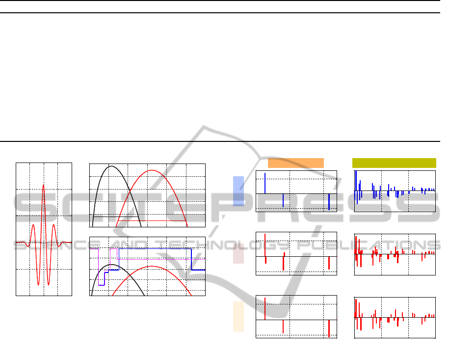
2.3 Comparison
The sinusoidally modulated Gaussian pulse used for
intra vehicular UWB channel sounding (Section 3)
has the form
x(t) =
s
2
√
2
t
d
√
π
exp
"
−

t
t
d

2
#
cos(2πf
c
t + φ) (1)
having unit energy, initial phase φ = 0.6π, and an ef-
fective pulse duration of 2t
d
= 0.276ns on either side.
The carrier frequency, f
c
= 6.5GHz, was set at the
middle of the FCC approved band (3GHz to 10GHz).
From Figure 1, it is easy to understand the rationale
behind choosing a Gaussian sine pulse over the popu-
lar Gaussian doublet: a flatter spectrum (-20 dB band-
width is almost 1.5 times), reduced low-frequency
components which aids antenna radiation, and a bet-
ter compliance with the outdoor and vehicular radar
UWB emission masks. The arguments hold true for
CLEANAlgorithmsforIntra-vehicularTime-domainUWBChannelSounding
225

Algorithm 2: Modified CLEAN.
STEP 01: compute cross-corrlation: R
xy
= x[n]
˜
∗y[n]
STEP 02: compute auto-corrlation: R
xx
= x[n]
˜
∗x[n]
STEP 03: initialize dirty map: d
0
← R
xy
, clean map: c
0
← 0 , threshold: T ← max|R
xy
|/10 ,
stopping criterion:
d
∗
0
← T + ε , N ← length {y}
STEP 04: while |d
∗
k
| > T do
find n
∗
k
=
arg max
n
|d
k
[n]|
, d
∗
k
← d
k
[n
∗
k
]
shift
auto-correlation R
xx,s
[n] = R
xx
[n+n
s
k
]
; n
s
k
= N −n
∗
k
clean
dirty map: d
k
← d
k−1
−d
∗
k
R
xx,s
if (0 < n
s
k
)
update
clean map: c
k
[n
s
k
] ← d
∗
k
end if
end while
STEP 05: return
ˆ
h ←c
      
-120
-115
-110
-105
-100
-95
Magnitude [dB]
-20 dB BW
= 4.65 GHz
-20 dB BW
= 7 GHz
0 2 4 6 8 10 12
-80
-70
-60
-50
-40
-30
Outdoor/ handheld
Vehicular radar
Frequency [GHz]
ESD [dBm / MHz]
-0.4 -0.2 0 0.2 0.4
-1
-0.5
0
0.5
1
1.5
x 10
5
Time [ns]
Amplitude [V]
Figure 1: Input pulse x(t) [left], it’s amplitude spec-
tra X( f) [right-top], and compliance with FCC UWB
emission masks [right-bottom]. The black curves depict
the frequency-domain characteristics for the Gaussian 2nd
derivative with equivalent parameters (unit energy and same
t
d
).
other baseband pulses too (e.g. raised cosine pulse
that obey Nyquist criterion).
For comparison, we have convolved the input
signal given in (1) with some energy normalized
(
∑
n
h
2
[n] = 1) synthetic impulse response, added
Gaussian noise, and applied the algorithms described
in Section 2.2 to estimate the CIRs. Although, the
common strategy is to match the reconstructed sig-
nal ˆy(t) against the original received signal y(t), we
compared
ˆ
h(t) directly with h(t) to see which method
provides better representation of the multipath nature
of the channel.
The test is first performed for a simple 3 tap chan-
nel with tap gains separated by a distance less than the
pulse width. A casual inspection of the reconstruc-
tion results (Figure 2 [left]) reveals that the modified
method results less spurious components, and the ra-
tio between CIR taps are better maintained.
Next we simulated the discrete version of the stan-
dard UWB IEEE 802.15.3 channel based on modified
0 0.5 1
-0.5
0
0.5
Original
3 Tap Channel
0 0.5 1
-0.5
0
0.5
Basic
0 0.5 1
-0.5
0
0.5
Modified
Time [ns]
0 5 10 15
-0.5
0
0.5
IEEE 802.15.3 Channel
0 5 10 15
-0.5
0
0.5
0 5 10 15
-0.5
0
0.5
Time [ns]
Figure 2: Comparison of the estimated CIRs with the origi-
nal CIR (SNR = 10dB, γ = 0.02).
Saleh-Valenzuela model (Molisch et al., 2003). The
simulation parameters for CM1/CM2 (0-4 m) were
assumed to resemble the intra-vehicular environment,
and only significant paths within 10dB of the peak
have been retained. Comparison of the estimated
CIR profiles (Figure 2 [right]) is no longer possible
through visual inspection. In fact, assessing relative
merits of two solutions for an ill-posed problem is
subjectiveto the metric used. For example, measuring
the number of significant MPCs is not very meaning-
ful, the multipath profile depends not only on num-
ber of taps, but also on their respective delays. An-
other crude method is to compare the mean square
error (MSE),
∑
N
n=1
(
ˆ
h[n] −h[n])
2
/N. However, the re-
sults averaged over 1000 channel samples indicated
marginal improvement (3-4%) of the MSE.
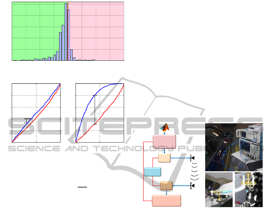
A better conclusion may be reached by resorting
to statistical comparisons. The parameter we use here
is Kullback-Leibler (KL) divergence
PECCS2015-5thInternationalConferenceonPervasiveandEmbeddedComputingandCommunicationSystems
226

-2 -1.5 -1 -0.5 0 0.5 1 1.5 2
0
0.05
0.1
0.15
0.2
0.25
d
MC
- d
BC
Frequency
d
BC
> d
MC
d
BC
< d
MC
0 0.5 1
0
0.2
0.4
0.6
0.8
1
p
BC
p
MC
p
Empirical CDF
0 0.5 1
0
0.2
0.4
0.6
0.8
1
p
BC
p
MC
p
Empirical CDF
Figure 3: [Top] Histogram of difference of KL distance.
[Bottom] Comparison of CDF of p-values for γ = 0.02 and
γ = 0.03.
d =
N
∑
n=1
h[n]log
2

h[n]
ˆ
h[n]

(2)
which measures the distance between common non-
zero elements of the CIR vector. Note that the suffixes
(BC and MC) are used to signify the basic CLEAN
and modified CLEAN algorithms.
A negative skewness of the histogram (Figure 3
[top]) of the difference of the distances vouch for the
superiority of the modified algorithm. The plot por-
trays, how often, on an average, the CIRs constructed
with the modified algorithm differ less than that ob-
tained through the basic algorithm.
Next, we performed a two-sample Kolmogorov-
Smirnov test. The test is different from the earlier
test in the sense that it does not judge the one-to-one
correlation, rather it focuses on the similarity of the
inherent random distribution of CIR tap gains. The
Kaplan-Meier estimate of the cumulative distribution
function (CDF) of the p-values, measured against a
5% significance level, are shown in Figure 3 [bot-
tom]. The CDF for the basic algorithm exceeds the
modified one, implying that the probability of obtain-
ing smaller p-values for the basic case is more. The
sensitivity of the basic algorithm to parameter setting
is also quite self explanatory. When the loop gain (γ)
changes slightly from 0.02 to 0.03, the gap between
the CDFs widens drastically.
3 MEASUREMENT SETUP AND
RESULTS
The UWB time domain channel sounding measure-
ments were performed in a mid-sized passenger car
Skoda Octavia III under static (not moving) condi-
tion. The Gaussian sine pulse generated through
the Tektronix AWG70002A waveform generator was
first amplified through a high power amplifier (HPA)
before feeding the signal to a wideband conical
monopole antenna. At the receiver side an identical
antenna is placed which receives the signal. The sig-
nal is then amplified through a low noise amplifier
(LNA) and viewed/ stored in a digital sampling oscil-
loscope Tektronix DPO72004C. Figure 4 depicts the
interconnections of the apparatus and close-ups of an-
tenna positioning.












 

!
"#!



Tektronix
DPO72004C





 !
 "
 
#
$%&%%
Figure 4: [Clockwise from left] Block diagram of the mea-
surement setup, picture of the apparatus, and antenna close-
ups (tripod and right windscreen).
As shown in Figure 5, a total of 52 different Tx-
Rx antenna positions, with separations ranging from
0.56m to 1.9m, were tested with different degrees of
passenger occupancy. Some measurements were re-
peated to investigate temporal variation, which were
found to be negligible.
The received signal, y(t), for a particular measure-
ment can be represented as
y(t) = x(t)∗h
Tx,Ant
∗h(t)∗h
Rx,Ant
= x
ref
(t)∗h(t) (3)
where h
Tx,Ant
and h
Rx,Ant
are the impulse responses
of the transmitter (Tx) and receiver (Rx) antennas,
and x
ref
(t) = x(t) ∗h
Tx,Ant
∗h
Rx,Ant
is the reference in-
put template that was obtained by measuring the re-
sponse of the input x(t) in an anechoic chamber free
from reflectors/ diffractions. Next, multipath inten-
sity profiles were obtained by deconvolving the re-
ceived signals with the input template using the mod-
ified CLEAN algorithm. Samples of the post process-
ing of data is shown in Figure 6 for two indicative
CLEANAlgorithmsforIntra-vehicularTime-domainUWBChannelSounding
227

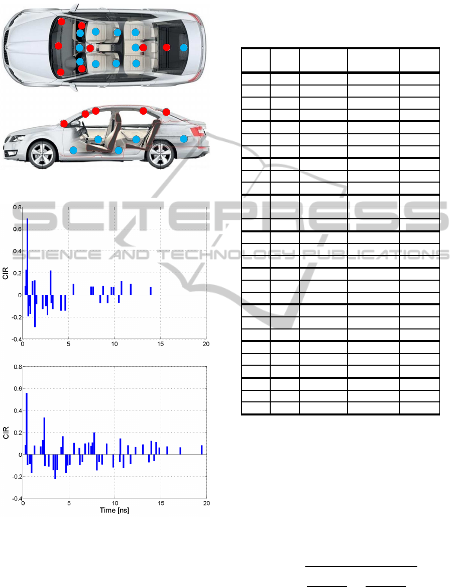
1R
5M
1M
1L
2L
2R
3R
3L
4R
4M
4L
1R
1M
1L
2L
2R
3M
4M
5M
1
2
3
4
5
1
2
3
4
5
Figure 5: Antenna placement in the car, RED: Tx antennas,
BLUE: Rx antennas.
Figure 6: Extracted CIR for LoS (Tx: 2L, Rx: 2R) condition
[Top] and nLoS (Tx: 2L, Rx: 4R) condition [Bottom].
cases with no passengers and the Tx antenna set at the
left side of the windscreen near the roof (2L in Figure
5); first when Rx antenna is placed on a tripod on the
driver seat (2R in Figure 5) creating a direct line-of-
sight (LoS) propagation path and next for a non-LOS
(nLoS) transmission with the Rx antenna on the rear
passenger seat on right (4R in Figure 5) with simi-
Table 1: Variation of RMS delay spread with passenger oc-
cupancy. Tx and Rx antenna positions are as per markings
in Figure 5. Passenger legends are, D: driver, FP: front pas-
senger, RL: rear passenger on left.
Rx Tx Tx-Rx Passenger τ
rms
pos. pos. gap [cm] [ns]
4R 1L 182 – 6.8880
” ” ” D 6.3442
” ” ” D, FP 5.6712
” ” ” D, FP, RL 4.9847
” 2L 146 – 5.8361
” ” ” D 5.1931
” ” ” D, FP 4.6487
” 1R 162 – 9.4691
” ” ” D 8.4802
” ” ” D, FP 7.8969
” 2R 119 – 7.9445
” ” ” D 7.9668
” ” ” D, FP 7.4689
” 5M 83 – 3.4871
” ” ” D 2.7340
” ” ” D, FP 2.9521
2R 4M 123 – 6.1866
” ” ” FP 5.6423
” ” ” FP, RL 3.9350
” 5M 161 – 7.0158
” ” ” FP 6.1101
” ” ” FP, RL 5.1240
” 2L 97 – 2.6203
” ” ” FP 2.0125
” ” ” FP, RL 2.1586
” 1L 118 – 4.7816
” ” ” FP 3.9739
” ” ” FP, RL 3.4004
lar tripod arrangements. The number of MPC is quite
higher for the nLoS case as expected.
The CIR profiles obtained after the post-
processing via CLEAN can be utilized to extract var-
ious channel parameters such as number of MPCs,
mean excess delay, etc. Nevertheless, our discus-
sions here are limited to root mean square (RMS) de-
lay spread which is not much susceptible to apparatus
settings and synchronization. RMS delay spread is
defined as the second central moment of the average
power delay profile, and can be calculated through the
formula
τ
rms
=
v
u
u
t
∑
n
τ
2
n
|
ˆ
h
n
|
2
∑
n
|
ˆ
h
n
|
2
−
"
∑
n
τ
n
|
ˆ
h
n
|
2
∑
n
|
ˆ
h
n
|
2
#
2
(4)
where {τ
n
,
ˆ
h
n
} are the delay and gain associated with
the nth path.
PECCS2015-5thInternationalConferenceonPervasiveandEmbeddedComputingandCommunicationSystems
228

Interestingly, when RMS delay spread values were
examined for different Tx-Rx distances, only a weak
correlation was observed. On the other hand, as seen
from Table 1, τ
rms
decreased consistently with higher
passenger occupancy across all different Tx-Rx set-
tings. The reduction in delay spread can be accounted
for the obstruction and absorption of several MPCs by
human body.
4 CONCLUSIONS
In this paper, we investigated two versions of CLEAN
algorithm for estimating CIR in intra-vehicular UWB
channel sounding experiment. The efficacy of the
modified CLEAN algorithm over the basic version
is established through statistical measures. Next, us-
ing the modified algorithm, post-processing of time
domain channel measurement data were performed.
The results show that while the RMS delay spread is
weakly dependent on the antenna separation, it de-
creases linearly with passenger occupancy.
We believe that CLEAN algorithms presented in
the current text would simplify human-computer in-
teractions for the wireless physical layer experimen-
talists, and would be appealing to those who are work-
ing towards realization of intelligent transportation
systems. Our project team is currently developing
a more sophisticated spread spectrum based channel
sounding system, and we would like to study the suit-
ability of these algorithms for the new setup.
ACKNOWLEDGEMENTS
This work was supported by the SoMoPro II pro-
gramme, Project No. 3SGA5720 Localization via
UWB, co-financed by the People Programme (Marie
Curie action) of the Seventh Framework Programme
of EU according to the REA Grant Agreement
No. 291782 and by the South-Moravian Region.
The research is further co-financed by the Czech
Science Foundation, Project No. 13-38735S Re-
search into wireless channels for intra-vehicle com-
munication and positioning, and was performed
in laboratories supported by the SIX project, No.
CZ.1.05/2.1.00/03.0072, the operational program Re-
search and Development for Innovation. The gener-
ous support from Tektronix, Testovac´ı Technika, and
Skoda a.s. Mlada Boleslav are also gratefully ac-
knowledged.
REFERENCES
Bas, C. U. and Ergen, S. C. (2013). Ultra-wideband chan-
nel model for intra-vehicular wireless sensor networks
beneath the chassis: from statistical model to simula-
tions. IEEE Trans. Veh. Tech., 62(1):14–25.
Bellens, F., Quitin, F., Dricot, J. M., Horlin, F., Benlarbi-
Dela¨ı, A., and Doncker, P. D. (2011). A wideband
channel model for intravehicular nomadic systems.
Int. J. Ant. Prop., 2011(468072):1–9.
Demir, U., Bas, C. U., and Ergen, S. C. (2014). Engine
compartment UWB channel model for intravehicular
wireless sensor networks. IEEE Trans. Veh. Tech.,
63(6):2497–2505.
Li, B., Zhao, C., Zhang, H., Sun, X., and Zhou, Z. (2013).
Characterization on clustered propagations of UWB
sensors in vehicle cabin: measurement, modeling and
evaluation. IEEE Sensors J., 13(4):1288–1300.
Liu, T. C. K., Kim, D. I., and Vaughan, R. G. (2007).
A high-resolution, multi-template deconvolution algo-
rithm for time-domain UWB channel characterization.
Can. J. Elect. Comput. Eng., 32(4):207–13.
Molisch, A. F., Jeffrey, R. F., and Marcus, P. (2003). Chan-
nel models for ultrawideband personal area networks.
IEEE Wireless Commun., 10(6):14–21.
Muqaibel, A., Safaai-Jazi, A., Woerner, B., and Riad, S.
(2002). UWB channel impulse response characteriza-
tion using deconvolution techniques. In Proc. IEEE
MWSCAS, volume 3, pages 605–08, Tulsa, OK, USA.
Niu, W., Li, J., and Talty, T. (2009). Ultra-wideband channel
modeling for intravehicle environment. EURASIP J.
Wirel. Commun. Net., 2009(806209):1–12.
Vaughan, R. G. and Scott, N. L. (1999). Super-resolution of
pulsed multipath channels for delay spread character-
ization. IEEE Trans. Commun., 47(3):343–47.
Yang, W. and Zhang, N. (2006). A new multi-template
CLEAN algorithm for UWB channel impulse re-
sponse characterization. In Proc. IEEE ICCT, pages
1–4, Guilin, China.
CLEANAlgorithmsforIntra-vehicularTime-domainUWBChannelSounding
229