
PRIAR using a Graph Segmentation Method
M. Righi
1,3
, M. D’Acunto
1,2,3
and O. Salvetti
1,3
1
ISTI-CNR, via Moruzzi 1, 56124, Pisa, Italy
2
ISM-CNR, via Fosso del Cavaliere, 100, 0133, Roma, Italy
3
NanoICT Laboratory, Area della Ricerca CNR Pisa, Pisa, Italy
Keywords:
Pattern Recognition, Image Analysis, Image Segmentation, Boundary Detection, Graph Partitioning Algo-
rithm.
Abstract:
Recently, we have suggested a simple and general-purpose method able to combine high-resolution analysis
with the classification and identification of components of microscopy imaging. The method named PRIAR
(Pattern Recognition Image Augumented Resolution) is a tool developed by the authors that gives the possi-
bility to enhance spatial and photometric resolution of low-res images. The implemented algorithm follows
the scheme: 1) image classification; 2) blind super-resolution on single frame; 3) pattern-analysis; 4) recon-
struction of the discovered pattern.
In this paper, we suggest some improvements of the PRIAR algorithm, in particular, the definition of a seg-
mentation method which is based on homomorphism between a processed image and a graph describing the
image itself, able to identify object of interest in complex patterns. The case study is the identification of
organs inside biological cells acquired with Atomic Force Microscopy Technique.
1 INTRODUCTION
Microscope image analysis is used in many fields of
technology, science and medicine. In all these appli-
cations, a common problem is represented by the low
resolution of objects of interest, so that detection and
classification are difficult and, because of correspon-
dent poor resolution, analysis of such objects can be
lead to misunderstanding. As a consequence, pattern
recognition (PR) and identification of objects of in-
terest is a first necessary step in order to improve the
quality of image analysis, the second step is to im-
prove the resolution from low level to high level, or
equivalently, multiple scale resolution.
PR applied to the imaging techniques is a term de-
noting supervision methods developed by the combi-
nation of machine learning, artificial intelligence and
data mining. PR methods can be categorized accord-
ing to the type of learning procedure used to generate
output value from input images. For example, super-
vised learning procedure assumes that a set of train-
ing data has been previously provided (Gonzalez and
Woods, 2008). Then, a further learning processing
generates a model that attempts to meet two general
requests: i), perform as well as possible on the train-
ing data, and, ii) generalize as well as possible to new
data or other input images. The other one category
is represented by the unsupervised learning methods.
This class of pattern recognition methods assumes
training data that has not been previously labelled,
and try to find inherent patterns in the data that can
be used to identify a correct output value for new data
instances (Theodoridis et al., 2008). A combination
of the two categories is also possible, mixing labelled
and unlabeled data in suitable ways, depending by the
data in input, and where the data to be labelled is the
training data (Bishop, 2006). Most common pattern
recognition algorithms are probabilistic in nature, in
that they use statistical inference to find label for a
given instance. In many applications, many proba-
bilistic algorithms output a list of n-best labels with
associated probabilities, instead of simply best label.
For example, PR can be used for classification, which
attempts to assign each input value to one of a given
set of classes, in this case, the n-best labels should be
fairly small (a binary choice for n is the best, yes or
not, 1 or 0, etc). All the microscopic techniques re-
quire highly sophisticated pattern recognition super-
vised methods, for example PR is crucial for the seg-
mentation procedure of components to be identified
and classified in a large image. Since PR strategies
are strongly dependent by the application, we focused
46
Righi M., D’Acunto M. and Salvetti O..
PRIAR using a Graph Segmentation Method.
DOI: 10.5220/0005461600460052
In Proceedings of the 5th International Workshop on Image Mining. Theory and Applications (IMTA-5-2015), pages 46-52
ISBN: 978-989-758-094-9
Copyright
c
2015 SCITEPRESS (Science and Technology Publications, Lda.)

the attention on methods connected to the identifica-
tion or organs and components inside biological sys-
tems like animal cells. For example, systemic analy-
sis of subcellular protein localization provides a key
for understanding gene functions and physiological
condition of the cells. However, recognition of cell
images of subcellular structures highly depends on
experience and becomes the rate-limiting step when
classifying subcellular protein localization. Several
research groups have extracted specific numerical fea-
tures for the recognition of subcellular protein local-
ization, but these recognition systems are restricted to
images of single particular cell line acquired by one
specific imaging system and not applied to recognize
a range of cell image sources.
Our imaging technique is based on the scanning
probe microscope (DAcunto, 2011), a technique that
measures the cells touching them with a probe ap-
proaching a resolution on the nanometer scale. On
the contrary, with respect to other microscope tech-
nique, like for example, the confocal microscopy, the
interaction between the microscopic tip probe and the
sample is limited to the cell cytoskeleton, i.e., the cell
surface, so pattern recognition methods must be ad-
dressed to identify skeleton components, like micro-
tubules, microfilaments, intermediate filaments, etc.
Once a skeleton components is identified, a proce-
dure of super-resolution (enhanced resolution) could
improve the data analysis and mining. The problem
of enhancing resolution of a single image refers to the
task of obtaining a high-resolution enlargement of a
single low resolution image, commonly recognised as
single-frame super-resolution problem. This problem
is intrinsically ill-posed because are generally multi-
ple frame images that can be combined to obtain final
high-resolution images. Accordingly to enhancing
resolution for a single image, strong prior information
must be realized. This information is available either
in the explicit form of a distribution defined on an im-
age class, or an implicit form of an example image
which leads to example-based super-resolution image
(Kim and Kwon, 2010). One diffuse approach for
the super-resolution of low-resolution image has been
characterized by algorithms including nearest neigh-
bour (NN)-based estimation. In such approach, there
are two distinct steps, in the first one, pairs of low-
resolution and corresponding high-resolution image
patches are collected. Then in the second one, the
super-resolution step, each patch of the given low-
resolution is contrasted to the stored low-resolution
patches, and the high-resolution patch corresponding
to the nearest low-resolution patch and satisfying a
certain spatial neighbourhood similarity can be evi-
denced so that can be considered as the final output of
the super-resolution image.
2 PRIAR 1.0: BASIC
FUNCTIONALITIES
The PRIAR (Pattern Recognition Image Augumented
Resolution) is a tool we have developed that gives the
possibility to enhance the resolution of low resolu-
tion images. It enhances the spatial resolution and
the depth of the image. The implemented algorithm
follows the scheme: 1) image classification; 2) blind
super-resolution on single frame; 3) pattern-analysis;
4) reconstruction of the discovered pattern. PRIAR
runs on Matlab 2013b, and the main features of the
computer used to test the program follows:CPU In-
tel(R) Core(TM) i5-2400 CPU @ 3.10GHz (4 cores)
with a L2 cache of 6144 KB with 16GB of RAM. The
program has been developed as mono-task, the idea
is to have a pipe-flow where each piece calculates a
subproblem sequentially. PRIAR works with in in-
put a low-resolution image and produces in output a
high-resolved computed image where the objects to
be identified are recognized and substituted with their
correspondent models. The execution time depends
on the size of the input data. A typical execution time
for patch images of 128 ×128 pixels, 8 bit per pixel,
is of about 70 seconds. The occupied memory de-
pends on the image size, the presented typical exam-
ple need of about 256 MB of RAM. The Matlab code
that describes algorithm implementation is detailed
elsewhere (Righi, 2014), here, we resume the basic
functions included inside with the following pseudo-
code:
01 Function [path enhanced_image]=PRIAR(input_image)
02 class=classification(input_image)
03 switch class
04 case:grating
segmentation_type=otsu
05 case:cell
segmentation_type=edge_discover
06 end
07 sr_image=blind_sr(input_image)
08 initial_path=
PRIAR-S(seed,super_resolved_image)
09 edge_discovered=
edge_discover(sr_image,segmentation_type)
10 path=
explore_extend(initial_path,segmented_image);
11 enhanced_image =build_model(sr_image,class)
12 end
The algorithm models a general purpose method to
analyse the images, in fact it uses a modular solu-
tion that permits to extend the class of the recog-
nized images and the image enhancement. The line
02 of the pseudo-code calls a data-mining function
PRIARusingaGraphSegmentationMethod
47

that classify the input image. In this particular imple-
mentation the function distinguish only two classes
of images: images representing a grating and im-
ages representing cells. The classification is impor-
tant during the next stages to choose the better seg-
mentation to adopt. The line 07 reports the function
call that super-resolve the image. During this step
the analysed image (that is a low resolution image)
is improved by increasing the colorimetric and spa-
tial resolution. The PRIAR implements the following
SR algorithms: Kim-Kwon (Kim and Kwon, 2010),
spline interpolation (Sonka et al., 2007), nearest-
neighbor interpolation (Ikonen and Toivanen, 2005),
bilinear interpolation (Bourke, 2001), bicubic inter-
polation (Getreuer, 2011), box-shaped kernel interpo-
lation (Ardizzone, 2009), Lanczos-2 kernel interpola-
tion (Getreuer, 2011) and Lanczos-3 kernel interpo-
lation (Ardizzone, 2009). The line 08 describes the
first step to map the object of interest (microtubule).
In each case, it needs a seed. The seed can be simply
a point of the object we are going to map or a poly-
line that follows a part of the object we are going to
discover. This is the algorithm we are going to de-
scribe in detail in the next sections. The main idea
of the explore algorithm is to crawl the surface until
certain parameters are respected. The role of the pa-
rameters can be summarized in the fact that the gap
between two next pixel must be enough small. At the
end of this exploration we have an initial path that
is a subset of the object we are going to trace. The
hypothesis that the initial path is a subset of the fi-
nal path is guarantee by the strong constraint that are
applied by the explore algorithm. The complexity of
this algorithm is linear with the number of the pixel
that composed the matrix. The explore algorithm per-
forms a local exploration so it is a local search al-
gorithm. Line 09 shows the edge discover function
call. The function used with grating images is differ-
ent by the one adopted with cell images in order to
avoid unwanted shadows. In fact, in order to edging
the grating super-resolved image, we combine the So-
bel method (Gonzalez and Woods, 2008; Gonzalez et
al., 2010), the Prewitt method (Gonzalez and Woods,
2008; Gonzalez et al., 2010), the Roberts method and
the Laplacian of Gauss method (Gonzalez and Woods,
2008; Gonzalez et al., 2010). If the we are analyzing a
cell image, we combine the Canny method (Gonzalez
and Woods, 2008; Gonzalez et al., 2010), the Zero-
Cross method (Gonzalez and Woods, 2008; Gonzalez
et al., 2010) and the previous listed methods.
3 PRIAR 1.1: IMPROVEMENTS
OF PRIAR WITH GRAPH
SEGMENTATION METHOD
In this section, we put in evidence the procedure un-
derlining the line 08 of PRIAR algorithm: i.e., the
identification of tyhe object of interest trough the seg-
mentation based on graph approach. Image segmen-
tation represents a challenge in image analysis. The
kind of segmentation that is required depends on user
objectives so different definitions and criteria have
been developed for image segmentation. Here, we
put in evidence a new method to segment a particu-
lar area of a gray-scale image,as previously identified
inside PRIAR procedure.
We represent the image with a proximity graph
where each node is associated to one image pixel. The
edges are labelled and reflects the neighbour relation
between pixels. Weights of edges is computed by a
function based on properties of corresponding pixel
such as the color intensity and the position. Accord-
ing to this representation the graph is used to deter-
mining the image segments. Let us consider a non-
oriented weighted graph G = (V, E,W) where V is the
set of the vertex that represents the image pixels, E the
edges that connect the vertex and the weighted edges
W represent the relationships between neighbour pix-
els. The weight matrix w
i j
, where i, j ∈ I where I
is the image, is a symmetric matrix. The use of the
image segmentation reduces the problem to a graph
clustering problem, in fact an image segment corre-
sponds to partition of the graph: the nodes of a par-
tition are strongly connected while the nodes that be-
longs to different partitions are weakly connected.
The application of a graph clustering algorithm to
a proximity graph will partition it into sub-graphs, the
objective of this research is to identify a single object
in an image so the PRIAR 1.1 algorithm will take in
account only a sub-graph. This paper extends the al-
gorithm described in (Righi et al., 2014; DAcunto et
al., 2015).
3.1 Image Representation
The graph G = (V, E,W ) represents the input image
where each node V represents a pixel of the source
image and the weight w
i j
is the distance between two
nodes. The distance between two nodes corresponds
to the distance between the the pixel i and the pixel j.
Since we want to recognize pixels that are in the same
segment, the weight of the graph represent the color
similarity and it is calculated by a likelihood func-
tion based on the local intensity of neighboring pixels.
IMTA-52015-5thInternationalWorkshoponImageMining.TheoryandApplications
48
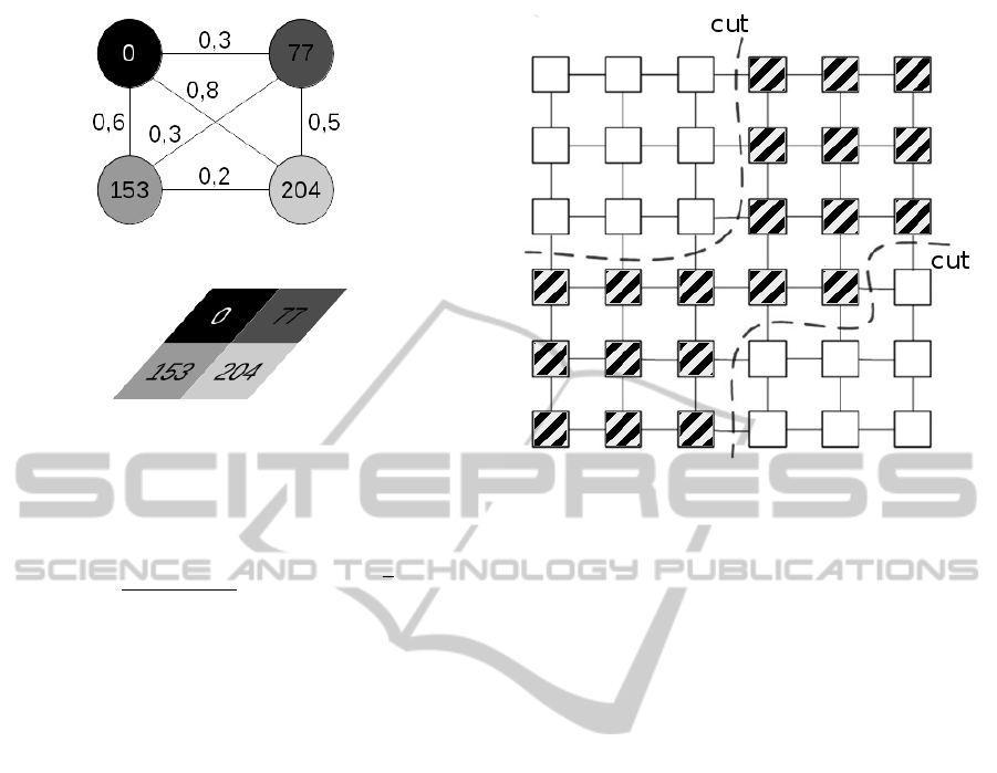
Figure 1: a portion of a 8-bit grayscale image and its asso-
ciated graph.
The weight are calculated as described in function 1.
w
i j
=
1 −
c
i
−c
j
max (c)
if d (i, j) ≤
√
2
0 otherwise
(1)
where d (i, j) is the Euclidean distance between pix-
els. There is an edge linking between two nodes only
if the nodes are close together. By using the weight of
function 1 next edges that have a close color belong
to the same structure: in this method of segmenting
a segment is determined by the homogeneity of the
color of pixels that constitute it. Figure 1 shows the
association between a portion of a 8-bit grayscale im-
age and its associated graph.
Note that by using this formulation the result can
be easily verified by a visual inspection of the image
searching homogeneous area of pixels.
A good result for a graph-based segmentation
methods depends on the translation of the color in-
formation of the source image into the graph: in order
to have an easily clusterization, the colour of a seg-
ment must be well separated from the color of other
segments. In order of improve the segmentation pro-
cedure, the image separation algorithm must use a
weighted function that is function of the input image.
This function is part of the image segmentation algo-
rithm and it is described into the next section.
3.2 Image Segmentation Algorithm
As described in section 3.1 an image can be repre-
sented by a proximity graph that can be crawled in
order to calculates a segment of interest. This method
implements the well-accepted criteria (Wertheimer,
Figure 2: an example of graph cuts and the corresponding
vertex weight.
1938) to recognize a segment. The segment of inter-
est is composed of strong bonds between the vertexes
that is surrounded by a set of weak bonds between
the vertexes. To find a segment in proximity graphs
of image, we use the graph as described in section
3.1. The key idea is that a segment is recognizable by
analysing neighbourhood relationships between ob-
jects in a particular space which reflects object sim-
ilarities. In most practical problems direct analysis is
unrealistic due to the high dimensionality of the space
(Peng et al., 2013) and it is necessary use an heuristic
approach to reduce the space where to search the goal
(Russell and Norvig, 2010). Our solution linearises
the search problem by reducing the algorithm com-
plexity to O(n) where n is the number of the pixel.
In this method the search problem is expressed by the
following relation:
cut (A, B) =
(
min
∑
i, j∈A
w
i j
max
∑
i∈A,i∈B
w
i j
(2)
where A is the segment we want recognize and B the
background. In figure 2, we show an example of such
graph cut. In order to segment the image it is used
min
∑
i, j∈A
as primary objective and max
∑
i∈A,i∈B
as
secondary objective. The idea to threat the segmen-
tation as an exploring game placing a crawler (the
player) on a vertex that is part of the interesting seg-
ment. The crawler can move from a vertex to another
one if there exists the condition to execute this move-
ment, the condition is a function of the input image.
Considering that the weights are constant, the crawler
can be implemented using a net surfer and a pixel
harvester. Both net surfer and pixel harvester pro-
PRIARusingaGraphSegmentationMethod
49
cedures are implemented using a deterministic finite
automaton. The net surfer is modelled by a IFA (It-
erated Finited Automa) (Zhang, 2008) and the pixel
harvester is modelled by a DFA (Deterministic Finite
Automaton) (Hopcroft and Ullman, 1969).
3.3 Net Surfer
The net surfer must navigate the graph in order to
have an exhaustive search over the graph. This task
is particularly important because it determines the al-
gorithm complexity: in fact the other function have a
linear complexity according to the size of the data in-
put. In order to maintain his algorithmic complexity
it is necessary that this task has an O(n) complexity
(Parinya et al., 2014; Zhang, 2008). The solution we
illustrate respect this constraint permitting us to have
a algorithm with linear complexity. The IFA is de-
fined by I = (S
i
, S
f
, S, I, A) where S
i
is the initial state,
S
f
is the final state, S are the non-terminal states and
A is the set of the actions. The nodes of I are homo-
morphic to G nodes, the operation performed by IFA
are used to calculated the next node that must be ex-
amined by the pixel harvester.
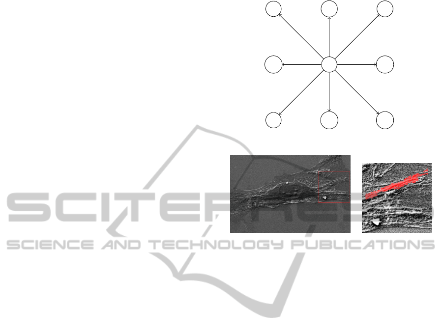
The input of the net surfer is a labelled graph G0=
(V, E) where each edge has a label from 1 to 8.
The IFA we use has a number of states that is
equivalent to the number of the vertex V of the G
graph. Each state stores two information: the last
edge that was visited and the belonging state value.
The belonging state value can be U,B or B:
• U means that it is a state that is not yet examined;
• B means that it is a state that corresponds to a ver-
tex that belongs to the segment;
• B means that it is a state that does not correspond
to a vertex that belongs to the segment.
We show in figure 3 the node label of the G0 graph.
The net surfer gets in input the first node and mark
its state as B, initializes the local variable of the node
edge counter with the value 1 and initialize the vari-
able history list of the nodes with the name of the first
node. The next step consists of the examination of
the variable value node edge to locate the next note
to analyse (the node at the end of the edge). If the
node has value U the net surfer calls the pixel har-
vester function (describe in sub-section 3.4) and ac-
cording to the pixel harvester answer change the state
of the node in B or B. If the state of the node is B
it will never analysed again. Otherwise the search of
the nodes that are in the segment continues from this
node assigning the state. Each time that a node is call
back it is increased its node edge by 1 and the search
a
b
c
d
e
f
g
h
i
1
2
3
4
5
6
7
8
Figure 3: the labelled graph G0 used by IFA.
A B
Figure 4: (a) the box emphatize the area where it is per-
formed the search (b) the filament tracked by PRIAR 1.1
algorithm.
starts again following the new edge. The search fin-
ishes when the variable node edge has reached the
value 9 and the history list contains only one node.
The returned value is a list of the pixels that are in the
segment.
3.4 Pixel Harvester
The pixel harvester evaluates the distance between
two pixels. Considering that ref(init) is the correspon-
dent value of the colour intensity between the first
node selected and its pixel, the adopted model con-
sider that the distance between two adjacent nodes i
and j are in the set B (the set of the nodes that are in
the segment) only if the equation 3 is satisfied.
i ∈B∧
ref (init) −w
i j
< v
1
∧w
i j
< v
2
⇒ j ∈B (3)
The constraints v
1
and v
2
depends on input data and
are inserted by the user.
3.5 Additional Results
PRIAR 1.1 algorithm gives has provided interesting
result during cell analysis. Here we show only two
samples where we put in evidence the features of the
algorithm (figures 4 and 5).
Moreover we tested our method by applying it
to synthetic images containing a set of cylindrical
IMTA-52015-5thInternationalWorkshoponImageMining.TheoryandApplications
50
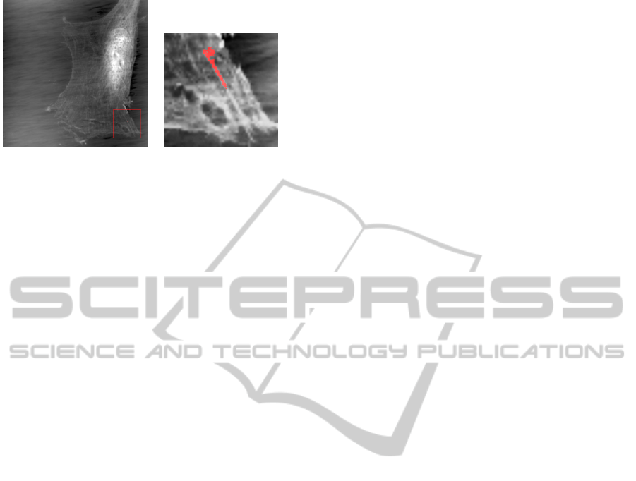
A B
Figure 5: (a) the box emphatize the area where it is per-
formed the search, (b) the filament tracked by using the
PRIAR 1.1 algorithm.
shapes. We found that these shapes could be recog-
nized after both reduction of resolution and addition
of noise. We found that the percentage error (num-
ber of pixels either wrongly assigned or non-assigned
to the pattern to identify) was 0.8 when the signal-to-
noise ratio was 11.6 dB and was 7.4 when the signal-
to-noise ratio was 8.7 dB.
4 CONCLUSIONS AND FUTURE
WORKS
In this paper, we have presented the PRIAR 1.1, a new
improved version of the code PRIAR (Pattern Recog-
nition Image Augmented Resolution)1.0. Essentially,
the new improvement regards the identification of ob-
ject of interest inside an image showing complex pat-
terns. The application is on stem cell cytoskeleton
recorded with an atomic force microscope. The key
idea is that the object of interest, (for example, a seg-
ment, that in the reality represents a cytoskeleton fil-
ament) is recognizable by analysing neighbourhood
relationships between objects in a particular space
which reflects objects similarities. Since, in most
practical problems, direct analysis is unrealistic due
to the high dimensionality of the space, we improved
the procedure linearizing the search problem by re-
ducing the algorithm complexity to O(n), where n is
the number of the pixel.
This method shows how the use of graphs to per-
form pattern-recognition is a powerful tool for the
recognition of objects in an image. Considering that
the same object can be isomorphic with more uncon-
nected subgraphs, we will study how to relate these
subgraphs and recognize when they refer to a single
object image.
ACKNOWLEDGEMENTS
The authors like to thank Serena Danti, Department
of Medicine, University of Pisa.
REFERENCES
Ardizzone, E. et al. (2009). Fuzzy-based kernel regression
approaches for free form deformation and elastic reg-
istration of medical images. In de Mello, C. A. B., ed-
itor, Biomedical Engineering. nTech.
Bishop, C. M. (2006). Pattern Recognition and Machine
Learning. Springer-Verlag New York, Inc.
Bourke, P. (2001). Bicubic Interpolation for Image Scaling.
DAcunto, M. (2011). Nanotribology and Biomaterials:
New Challenges for Atomic Force Microsopy. In Ad-
vances in Nanotechnology, Advances in Nanotechnol-
ogy, pages 105142. Nova Science.
DAcunto, M. et al. (2015). A new method combining En-
hanced Resolution and Pattern Identification. submit-
ted to The Open Medical Informatics Journal.
Getreuer, P. (2011). Linear Methods for Image Interpola-
tion. Image Processing On Line, 18.
Gonzalez, R. C. et al. (2010). Digital Image Processing
Using MATLAB. Prentice Hall, 2nd edition.
Gonzalez, R. C. and Woods, R. E. (2008). Digital image
processing. Prentice Hall, Upper Saddle River, N.J.
Hopcroft, J. E. and Ullman, J. D. (1969). Formal Lan-
guages and Their Relation to Automata. Addison-
Wesley Longman Publishing Co., Inc., Boston, MA,
USA.
Ikonen, L. and Toivanen, P. J. (2005). Distance and Nearest
Neighbor Transforms of Gray-Level Surfaces Using
Priority Pixel Queue Algorithm. In Blanc-Talon, J. et
al., editors, ACIVS, volume 3708 of Lecture Notes in
Computer Science, pages 308315. Springer.
Kim, K. I. and Kwon, Y. (2010). Single-Image Super-
Resolution Using Sparse Regression and Natural Im-
age Prior. IEEE Trans. Pattern Anal. Mach. Intell.,
32(6):11271133.
Parinya, C. et al. (2014). Pre-Reduction Graph Products:
Hardnesses of Properly Learning DFAs and Approx-
imating EDP on DAGs. In Foundations of Computer
Science (FOCS), 2014 IEEE 55th Annual Symposium
on, pages 444453. IEEE.
Peng, B. et al. (2013). A Survey of Graph Theoretical Ap-
proaches to Image Segmentation. Pattern Recogn.,
46(3):10201038.
Righi, M. (2014). Pattern Recognition Image Augmented
Resolution: a tool for image analysis. Technical Re-
port.
Righi, M. et al. (2014). PRIAR (Pattern Recognition Image
Augmented Resolution) a tool to combine pattern-
recognition with superresolution. In 9th International
Conference on Open German Russian Workshop on
Pattern Recognition and Image Understanding.
Russell, S. and Norvig, P. (2010). Artificial Intelligence: A
Modern Approach. Prentice Hall, 3 edition.
PRIARusingaGraphSegmentationMethod
51

Sonka, M. et al. (2007). Image Processing, Analysis, and
Machine Vision. Thomson-Engineering.
Theodoridis, S. et al. (2008). Pattern Recognition. Aca-
demic Press, 4th edition.
Wertheimer, M. (1938). Laws of organization in perceptual
forms. In Ellis, W., editor, A Source Book of Gestalt
Psychology, pages 7188. Routledge and Kegan Paul,
London.
Zhang, J. (2008). Complexity and Universality of Iterated
Finite Automata. Complex Systems, 18.
IMTA-52015-5thInternationalWorkshoponImageMining.TheoryandApplications
52
