Optimal Irrigation Scheduling and Crop Production Functions

Development using AquaCrop and TOMLAB

Ilya Ioslovich and Raphael Linker

Faculty of Civil and Environmental Engineering, Technion–Israel Institute of Technology, 32000 Haifa, Israel

Keywords:

Irrigation Scheduling, Optimal Control.

Abstract:

Water stress is one of the most inﬂuential factors contributing to crop yield loss. The importance of the irriga-

tion constantly increases because of water scarcity and growing demand for agricultural production worldwide.

Previously, an approach using empirical water production functions and analytic optimal control methodology

has been developed for optimal irrigation scheduling. Such an approach based on numerical optimal control

is an alternative to common irrigation scheduling based on agronomy practice. Nowadays, more complex

dynamic crop simulation models, such as the FAO AquaCrop model, predict crop responses to different irri-

gation strategies and climates. The state variables of the AquaCrop model include crop characteristics, such

as biomass, and soil water content in up to 12 soil layers. In this paper the numerical optimal control scheme

for irrigation scheduling and crop water production function development is described and demonstrated using

this model and the TOMLAB optimization library. Maize crop in Foggia, Italy, for season of the year 2000, is

used as an illustrative case study.

1 INTRODUCTION

In order to cope with increased water scarcity and

hence limited water supply, the development of meth-

ods to produce efﬁcient irrigation scheduling is an im-

portant task. Many studies were performed in this

area during decades. For instance, the effects of

the supplemental irrigation for wheat in the region

of Aleppo, North Syria, were investigated in (Oweis

et al., 2003) using the simulation model ISAREG.

Different water policies to cope with water shortage

were studied in (Amir and Fisher, 2000) for the case

of Jezreel Valley district, Israel, using linear program-

ming optimization model. Analytical optimal con-

trol was used in (Shani et al., 2004), (Shani et al.,

2009), (Ioslovich et al., 2012), in conjunction with

the simpliﬁed STZ model. This model has only two

state variables: biomass of the crop and water con-

tent of the soil. The harvest index HI (percent of

the yield to the biomass) was assumed to be constant.

No precipitation was considered and the climate in-

puts were assumed to remain constant. By compar-

ison, the FAO model AquaCrop described in (Ste-

duto et al., 2009), (Geerts et al., 2009), (Geerts et al.,

2010), (Heng et al., 2009), (Xiangxiang et al., 2013)

is much more detailed and mimics crop development

much more closely. This model has several mech-

anisms of stresses, up to 12 soil layers and accept

time-varying climate inputs. It has been used with

averaged statistical measurements for development of

crop-water production functions in (Garcia-Villa and

Fereres, 2012). However these data concerned the use

of the irrigation water were connected only with ex-

isting agronomic practice without any prospects on

its optimization. Model based optimization of irri-

gation scheduling with AquaCrop and genetic algo-

rithms has been presented in (Linker et al., 2013) for

cotton in the Northern Greece.

Here we consider the optimal control scheme for

maximization of the yield within given irrigation wa-

ter quota and development the crop-water production

function based on the set of these optimizations. The

example of a maize crop in the Foggia region, Italy,

season 2000 is presented.

2 PROBLEM FORMULATION

The considered formulation of the problem of optimal

irrigation scheduling is as follows:

J = Y(w

,...,w

) [t/ha] → max

+ w

+ ... + w

≤ w [mm]. (1)

Ioslovich I. and Linker R..

Optimal Irrigation Scheduling and Crop Production Functions Development using AquaCrop and TOMLAB.

DOI: 10.5220/0005501700490052

In Proceedings of the 12th International Conference on Informatics in Control, Automation and Robotics (ICINCO-2015), pages 49-52

ISBN: 978-989-758-122-9

 2015 SCITEPRESS (Science and Technology Publications, Lda.)

Here Y is a value of yield, w

is daily irrigation for

day i, and w is a seasonal irrigation water quota. This

is a discrete analog of the optimal control problem as

follows:

J =

(t,w(t),x(t),t)dt → max

= f(t,w(t),x(t)),

w(t)dt ≤ w. (2)

However the functions f

and f(t, w(t),x(t)) are not

known and only the value of the functional J in

response to the seasonal sequence of the irrigation

events w

can be obtained from the AquaCrop sim-

ulation.

The AquaCrop predicts the seasonal crop devel-

opment in response to environmental variables and

irrigation. By calculating the set of these solutions

with gradually decreasing seasonal water quota w we

can construct the crop-water production function y(w)

which can be used for planning purposes both by

farmers and by water authorities.

3 CROP MODEL

The FAO Aquacrop model is widely used by many

users including farmers, water managers and agri-

cultural consultants. It represents a good balance

between accuracy, simplicity and robustness. The

AquaCrop model adequately simulates the canopy

cover, evapotranspiration, yield, and water content in

the soil. It has been successively calibrated and tested

for different crops such as cotton, wheat, tomato,

potato at different locations. Several algorithms have

been included in the AquaCrop that allow the user to

generate irrigation scheduling based on triggering ir-

rigation at user-speciﬁed soil water contents, which

should be linked to crop growth stage via the user

agronomic considerations and experience. Many de-

tails concerning this model can be found in (Steduto

et al., 2009), (Geerts et al., 2009), (Geerts et al.,

2010), (Heng et al., 2009), (Mkhabela and Bullock,

2012), (Xiangxiang et al., 2013). Though the under-

lying principles of the AquaCrop are well described,

the source code of the model is not available to users,

and thus it can be used only as a sort of black-box

model.

4 OPTIMIZATION SOLVER

We are using the TOMLAB optimization library for

MATLAB, (Holmstrom et al., 2007), that contains

many optimization solvers. The best results were

obtained by the use of OQNLP solver in combina-

tion with the qlcAssign procedure for global nonlin-

ear search. A special interface with the AquaCrop

model software was designed and used. The OQNLP

solver realizes a smart multistart heuristic algorithm

in conjunction with smooth optimization to search

for a global optimum of nonlinear constrained opti-

mization. This approach requires that we supply the

solver with a program that calculates the nonlinear

objective function (yield in our case). This function

writes the irrigation schedule in the appropriate ﬁle,

runs the AquaCrop from MATLAB and then reads

the output ﬁle generated by AquaCrop. The linear

constraint which represents the total seasonal irriga-

tion water sum is used. Throughout the optimization

search, all intermediate improving and feasible results

were recorded and the best result was retrieved after

the predeﬁned number of iterations was reached. The

qlcAssign procedure handles problems of the form

c(x) → min

≤ Ax ≤ b

≤ x ≤ x

. (3)

The constraints b

are used as an upper limit for

daily level of the irrigation. Although AquaCrop

requires integer irrigation amounts, the optimiza-

tion was performed in continuous mode because the

mixed-integer option did not yield good results. In

order to do this we have used a scaling procedure by

multiplying the vector of irrigation values by 1E-6

before transferring it to the solver and then scaling

it back before transferring it to AquaCrop. The lin-

ear matrix of constraints has to be modiﬁed accord-

ingly. The rounding of the variables receivedfrom the

solver in ﬂoat format was done with a special stochas-

tic procedure which considers the non-integer part as

a value of a probability distribution function (PDF)

which generates values in the range 0− 1 from a uni-

form random numbers generator (MATLAB function

rand).

The choice of the initial point for optimization

plays an important role. We have used the approach

reported in (Linker and Ioslovich, 2015). This ap-

proach, which has proved to be very efﬁcient, gener-

ates sub-optimal irrigation schedules via optimal lev-

els of soil water depletion at which irrigation is trig-

gered.

ICINCO2015-12thInternationalConferenceonInformaticsinControl,AutomationandRobotics

5 OPTIMIZATION SCHEME

The optimization scheme for optimal irrigation

scheduling with the AquaCrop and OQNLP consists

of the following steps:

1. The initial point (seasonal irrigation sub-optimal

schedule is calculated).

2. The AquaCrop runs the initial irrigation schedule

and a special interface transforms the irrigation

schedule into initial data for OQNLP

3. The OQNLP starts and invokes the users non-

linear objective function. The objective function

writes the AquaCrop irrigation ﬁle, invokes the

AquaCrop, reads the AquaCrop output ﬁle, pro-

vides the OQNLP with objective function value,

and stores the values related to the best record.

4. The OQNLP generates the next optimization point

and continues until the given number of iterations

is exceeded or OQNLP ends the execution be-

cause the convergence criteria has been met.

6 CROP-WATER PRODUCTION

FUNCTION

The constraint related for the seasonal water quota is

gradually decreased and a set of optimizations is per-

formed. This way a number of points in the plane

w,Y is obtained. The convex hull of the set of these

points is constructed up to the point with maximal

Y and the points of the vertices of this hull are then

used to construct the crop-water production function

for this crop. A second-order polynomial is used to

ﬁt these vertices. Unlike e.g. in (Garcia-Villa and

Fereres, 2012) which used so-called ”best agronomic

practice” this production function represents the opti-

mal irrigation scheduling.

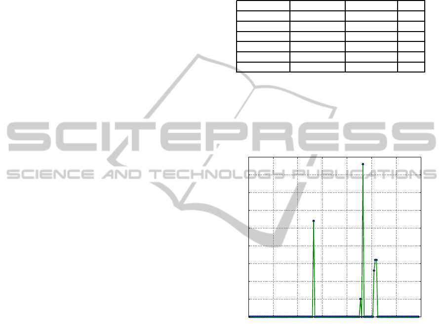
7 RESULTS FOR MAIZE IN

FOGGIA

The results for maize crop in Foggia region, Italy, sea-

son 2000, are shown in Fig. 1 and Fig.2. The simu-

lated period is 138 days long started on 22 of March

2000. Fig 1. represents the optimal irrigation sched-

ule for the water quota 120 [mm]. There are 5 irriga-

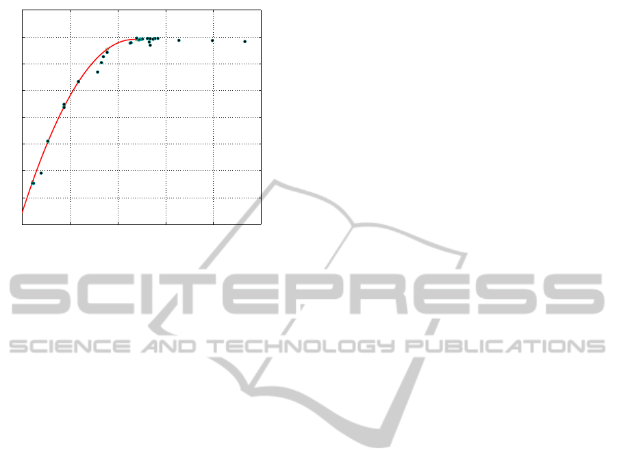
tion events throughout the season. The Fig. 2 shows

the crop-water production function together with the

convex hull vertices marked by ’*’, the approximated

points marked by ’o’, and suboptimal points marked

by ’+’. One can see that the mean increase in yield

gives about 10 [kg/ha] of yield per 1 [mm] of irriga-

tion. The table 1 shows the data corresponding to the

basic points.

Table 1: Basic points of the crop-water production function

for seasonal irrigation. Maize irrigation in Foggia, 2000.

Basic point Quota [mm] Yield [t/ha] HI

1 11 11,506 48,3

2 27 11,821 48,3

3 44 12,095 48,3

4 59 12,266 48,4

5 89 12,483 48,3

6 120 12,588 48,3

One can notice that the harvest index HI is rather

the same for all the basic points, which indicates

that while the biomass is limited by the water quota,

the value of the yield for the optimal irrigation takes

rather the same part of the total biomass for different

quotas.

0 20 40 60 80 100 120 140

Days after planting

Irrigation [mm]

Figure 1: Optimal irrigation scheduling for seasonal irriga-

tion quota 120 [mm]. Maize in Foggia, Italy, year 2000.

Irrigation levels marked as ’o’.

8 CONCLUSIONS

The optimization of the irrigation scheduling may be

performed using the optimal control scheme and the

Aquacrop model as demonstrated in this paper. The

agronomic knowledge is already incorporated in the

model and can be used in a limited way by supply-

ing of the reasonable initial point for these calcula-

tions. The crop-water production functions can be

developed based on the optimal irrigation scheduling

for different water quotas. This approach has been

demonstrated for a maize crop in the Foggia region,

Southern Italy, season 2000.

OptimalIrrigationSchedulingandCropProductionFunctionsDevelopmentusingAquaCropandTOMLAB

0 50 100 150 200 250

11.2

11.4

11.6

11.8

12.2

12.4

12.6

12.8

Irrigation water

Yield

Figure 2: Crop-water production function. Yield [t/ha] vs.

irrigation water [mm]. Maize in Foggia, Italy, year 2000.

Suboptimal points marked as black ’o’, basic points of the

convex hull marked as ’*’, points from quadratic approxi-

mation marked as ’o’.

ACKNOWLEDGEMENTS

The research leading to these results has received

funding from the European Community’s Seventh

Framework Programme (FP7/2007-2013) under grant

agreement n 311903–FIGARO (Flexible and Pre-

cise Irrigation Platform to Improve Farm-Scale Water

Productivity) (http://www.ﬁgaro-irrigation.net/). The

contents of this document are the sole responsibility

of the FIGARO Consortium and can under no cir-

cumstances be regarded as reﬂecting the position of

the European Union. This Research was supported

by Technion General Research Fund.

REFERENCES

Amir, I. and Fisher, F. (2000). Response of near optimal

agricultural production to water policies. Agricultural

Systems, 64:115–130.

Garcia-Villa, M. and Fereres, E. (2012). Combining the

simulation crop model AquaCrop with an economic

model for the optimisation of irrigation management

at farm level. European Journal of Agronomy, 36:21–

31.

Geerts, S., Raes, D., and Garcia, M. (2010). Using

AquaCrop to derive deﬁcit irrigation schedules. Agri-

cultural Water Management, 98:213–216.

Geerts, S., Raes, D., Garcia, M., Miranda, R., Cusicanqui,

J., A., Taboada, C., Mendoza, J., Huanca, R., Mamani,

A., Condori, O., Mamani, J., Morales, B., Osco, V.,

and Steduto, P. (2009). Simulating yield response of

Quinoa to water availability with AquaCrop. Agron-

omy Journal, 101:499–508.

Heng, L. K., Hsiao, T., C., S, E., Howell, T., and P, S.

(2009). Validating the FAO AcuaCrop model for irri-

gated and water deﬁcient ﬁeld maize. Agronomy Jour-

nal, 101:488–498.

Holmstrom, K., Goran, A., O., and Edvall M., M.

(2007). Users Guide for TOMLAB/OQNLP.

http://tomopt.com/tomlab/products/oqnlp/.

Ioslovich, I., Borshchevsky, M., and Gutman, P.-O. (2012).

On optimal irrigation scheduling. Dynamics of Con-

tinuous, Discrete and Impulsive Systems, Series B:

Applications and Algorithms, 19:303–310.

Linker, R. and Ioslovich, I. (2015). A multi-year simu-

lation study of optimal and sub-optimal irrigation of

maize in Kansas. In 2015 ASABE Annual Interna-

tional Meeting in New Orleans, Louisiana, USA, July

26-July 29. ASABE Online Technical Library.

Linker, R., Sylaos, G., and Ioslovich, I. (2013). Optimiza-

tion of irrigation scheduling using genetic algorithms

and AcuaCrop: a case study for cotton in Northern

Greece. In Proceedings of the International Confer-

ence on Agriculture Science and Environmental En-

gineering (ICASEE 2013), DVD. December 19-20,

Beijing, China, paper ICASEE 132117.

Mkhabela, M., S. and Bullock, P., R. (2012). Performance

of the FAO AcroCrop model for wheat grain yield and

soil moisture simulation in Western Canada. Agricul-

tural Water Management, 110:16–24.

Oweis, T., Rodrigues, P., N., and Pereira, L., S. (2003).

Tools for Drought Mitigation in Mediterranean re-

gions. Simulation of Supplemental Irrigation Strate-

gies for Wheat in near East to Cope with Water

Scarcity, pages 259–272. Kluwer Academic Publish-

ers.

Shani, U., Tsur, Y., and Zemel, A. (2004). Optimal dynamic

irrigation schemes. Optimal Control Applications and

methods, 25:91–106.

Shani, U., Tsur, Y., Zemel, A., and Zilberman, D. (2009).

Irrigation production functions with water-capital sub-

stitution. Agricultural Economics, 40:55–66.

Steduto, P., Hsiao, T., C., Raes, D., and Ferereset, E. (2009).

AcuaCrop the FAO crop model to simulate yield re-

sponce to water: I. concepts and underlying princi-

ples. Agronomy Journal, 101:426–437.

Xiangxiang, W., Quanjiu, W., Jun, F., and Quiping, F.

(2013). Evaluation of the AquaCrop model for sim-

ulating the impact of water deﬁcits and different ir-

rigation regimes on the biomass and yield of winter

wheat grown on China’s Loess Plateau. Agricultural

Water Management, 129:95–104.

ICINCO2015-12thInternationalConferenceonInformaticsinControl,AutomationandRobotics