
Extreme Learning Machines with Simple Cascades
Tom Gedeon and Anthony Oakden
Research School of Computer Science, The Australian National University, Canberra, ACT 2601, Australia
Keywords: Extreme Learning Machines, Cascade Correlation, Shallow Cascade, Simple Cascade, Full Cascade,
Cascade Extreme Learning Machine, Cascade ELM.
Abstract: We compare extreme learning machines with cascade correlation on a standard benchmark dataset for
comparing cascade networks along with another commonly used dataset. We introduce a number of hybrid
cascade extreme learning machine topologies ranging from simple shallow cascade ELM networks to full
cascade ELM networks. We found that the simplest cascade topology provided surprising benefit with a
cascade correlation style cascade for small extreme learning machine layers. Our full cascade ELM
architecture achieved high performance with even a single neuron per ELM cascade, suggesting that our
approach may have general utility, though further work needs to be done using more datasets. We suggest
extensions of our cascade ELM approach, with the use of network analysis, addition of noise, and
unfreezing of weights.
1 INTRODUCTION
Extreme learning machines (ELMs) are a fast way to
construct the output weights for single layer feed
forward neural networks, where the input layer of
weights is frozen. The output weights can be trained
using the delta rule, but it is quicker to use the
Moore-Penrose pseudo-inverse to estimate the
weights (Huang, et al., 2004). A thorough survey
can be found in Huang (et al, 2011). Beyond the
initial successes with the MNIST dataset, ELM
networks have been successfully used in various
application areas such as face recognition (Marques
and Graña, 2012), and to handle uncertain data (Sun,
et al, 2014).
Cascade correlation neural networks are a way to
grow narrow deep networks efficiently (Fahlman
and Lebiere, 1990). A layered cascade network has
been proposed and some initial good properties
shown (Shen and Zhu, 2012) and provides part of
the motivation for our work. Cascade correlation
freezes weights after each neuron is added, so only
new weights are trained, which has some obvious
similarities to ELM, if we could do this in a layered
fashion rather than neuron-by-neuron.
There is little prior art in the combination of
ELM and cascade correlation related structures. We
note there is some work on Echo State networks by
Yao (et al, 2013) which has some similarity. Echo
state networks were introduced by Jaeger (2001),
and use a similar algorithm to train recurrent and not
feedforward networks. See Bin (et al, 2011) for a
comparison of Echo State and ELM. We also note
that Wefky (et al, 2013) define cascade networks in
general as we define our shallow cascade network
topology, and Tissera and McDonnell (2015) use a
layered auto-associative structure which could be
described as a cascade network, though they do not
express this in their paper.
2 BACKGROUND
The most common neural network model is a multi-
layer feedforward neural network trained using the
back-propagation algorithm (backprop) (Rumelhart,
Hinton and Williams, 1986). It is generally accepted
that three layers of processing neurons are sufficient
to learn arbitrary mappings from the input to the
output given sufficient neurons in the intermediate
(‘hidden’) layers. It is possible to eliminate one of
the layers by accepting multiple outputs representing
the same output class, so two layers of processing
neurons are sufficient. Thus we have the output layer
and a single hidden layer. The key to supervised
learning in feed-forward networks is the error signal
derived from the difference between actual and
desired output weights, which is used to modify the
271
Gedeon T. and Oakden A..
Extreme Learning Machines with Simple Cascades.
DOI: 10.5220/0005539502710278
In Proceedings of the 5th International Conference on Simulation and Modeling Methodologies, Technologies and Applications (SIMULTECH-2015),
pages 271-278
ISBN: 978-989-758-120-5
Copyright
c
2015 SCITEPRESS (Science and Technology Publications, Lda.)

hidden-to-output weights to improve network
performance at each step. This error signal is then
estimated for each preceding layer, but the error
signal attenuates.
2.1 Extreme Learning Machine
Figure 1: Simple ELM network.
Huang et al’s (2004) principal contribution was to
suggest that a set of random weights in the hidden
layer could be used as a way to provide non-linear
mapping between the input neurons and the output
neurons. By having a large enough number of
neurons in the hidden layer the algorithm can map a
small number of input neurons to an arbitrarily large
number of output neurons in a non-linear way.
Training is performed only on the output neurons
and performance similar to multi-layer feed-forward
networks using back propagation achieved with
much reduced training time.
It is possible to train an ELM network as shown
in Figure 1 by using back-propagation, but since the
input-to-hidden weights are fixed, it is more efficient
to estimate the output weights using the Moore-
Penrose pseudo-inverse (Huang et al., 2004). The
weight matrix calculated is the best least square
error fit for the output layer and in addition provide
the smallest norm of weights, which is important for
optimal generalisation performance (Bartlett, 1998).
2.2 Cascade Correlation
The Cascade Correlation algorithm (Cascor)
(Fahlman and Lebiere, 1990) is a very powerful
method for training artificial neural networks.
Cascor is a constructive algorithm which begins
training with a single input layer connected directly
to the output layer. Neurons are added one at time to
the network and are connected to all previous hidden
and input neurons, producing a cascade network.
When a new neuron is to be added to the network,
all previous network weights are 'frozen'. The input
weights of the neuron which is about to be added are
then trained to maximise the correlation between
that neuron's output and the remaining network
error. The new neuron is then inserted into the
network, and all weights connected to the output
neurons are then trained to minimise the error
function.
Thus there are two training phases: the training
of the hidden neuron weights, and the training of
output weights. A previous extension to the cascor
algorithm was by the use of the RPROP (Riedmiller,
1994) algorithm to train the whole network
(Treadgold and Gedeon, 1997) with ‘frozen’ weights
represented by initially low learning rates. That
model (Casper), was shown to produce more
compact networks, which also generalise better than
Cascor.
2.3 Caveats
We have said it is generally accepted that 3 layers of
processing neurons is sufficient, but we must point
out that this is not always true.
For example, we know that in the field of
petroleum engineering, in order to reproduce the
fine-scale variability known to exist in core porosity/
permeability data, separate neural nets are used for
porosity prediction, followed by another for
permeability prediction. This produces better results
than a single combined network (Wong, Taggart and
Gedeon, 1995), and for hierarchical data (Gedeon
and Kóczy, 1998).
3 CASCADE CORRELATION
AND EXTREME LEARNING
MACHINE
ELMs can be trained very quickly to solve
classification problems. In general the larger the
hidden layer the higher the learning capacity of the
network. However the size of the hidden layer is
critical to performance. Too small and the network
will not have sufficient capacity to learn but too
large, learning times will suffer and over fitting
occurs.
Finding the ideal size for the layer is
problematic. If the number of neurons is greater or
equal to the number of training patterns then the
network will be able to achieve 100% learning.
However this is not a useful conclusion as in most
cases we would expect the network to achieve
satisfactory learning with far less neurons than this.
SIMULTECH2015-5thInternationalConferenceonSimulationandModelingMethodologies,Technologiesand
Applications
272
The random nature of the hidden layer further
exacerbates this problem of finding the ideal layer
size because depending on the random weights
added we may require more or less weights.
It would be convenient if we could start with a
relatively small number of weights, test the network
and if performance is substandard gradually add
more weights. In this section we explore some
simple modifications of the ELM architecture which
makes this approach possible.
3.1 Data Sets
The two spiral dataset consists of two interlocked
spirals in 2 dimensions (Kools, 2013), the network
must learn to distinguish the two spirals. This dataset
is known to be difficult for traditional backprop to
solve (Fahlman and Lebiere, 1990), and has the
advantage of being easy to visualise, hence we can
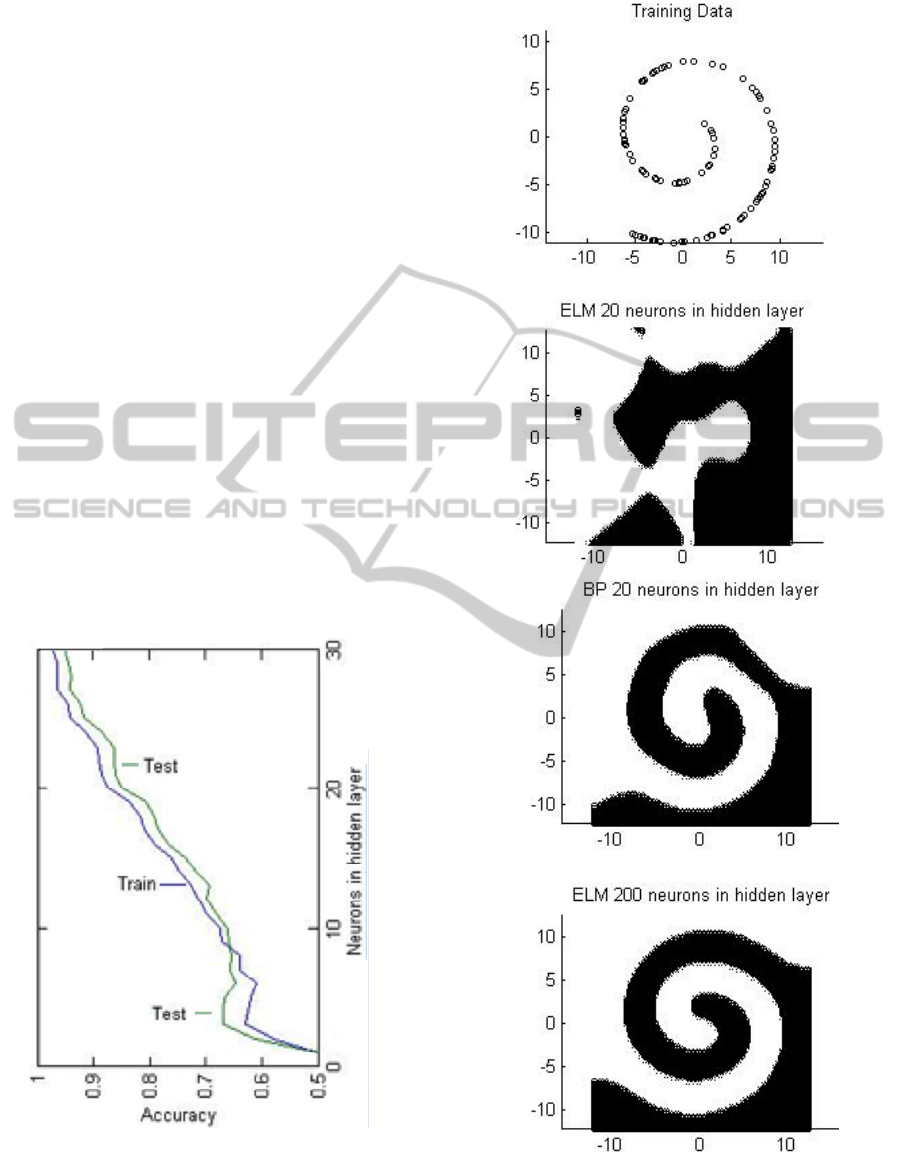
readily see the performance of a network, Figure 3.
With 20 hidden neurons, backprop produces a
good result, while ELM does not. With 200 hidden
neurons, ELM produces a slightly better result. With
our computer, the BP 20 result took 6.4 secs, while
the ELM 200 result took 0.06 secs, we found overall
that ELM was 15-100 times faster. As we can see in
Fig. 3, 30 or more hidden neurons are sufficient.
Figure 2: Comparison of train/test accuracy as ELM
hidden layer size increases.
Figure 3: Comparison of training results for double spiral
data set.
We also use the Pima Indians Diabetes Database
ExtremeLearningMachineswithSimpleCascades
273
from the UCI machine learning repository (Blake
and Merz, 1998). Good results on this dataset from
the literature using a number of AI techniques are in
the mid to high 70% range. Our ELM and cascade
ELM results fall in this range in general so we will
not compare our results to the literature in more
detail, as our focus is on the effects of introducing
cascades to ELM networks. We found similar results
with some other UCI datasets which we do not
report here.
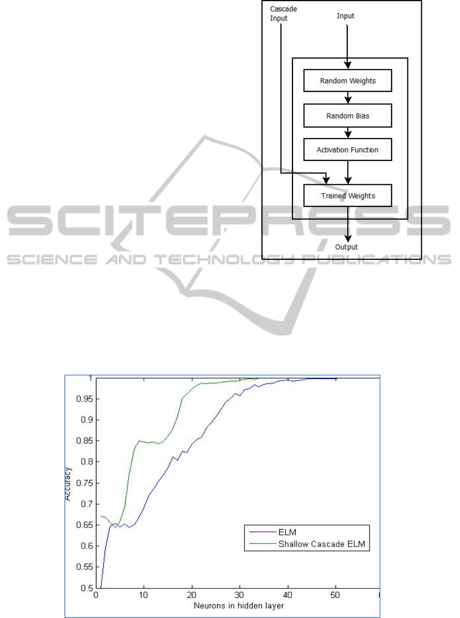
3.2 Shallow Cascade
The simplest modification is to connect the inputs
directly to the outputs as additional connections.
Cascade correlation starts with these connections,
hence adding these connections into the ELM
architecture as our first step is appropriate, see
Figure 4. These weights are then ‘trained’ using the
Moore-Penrose pseudo-inverse as before. The
performance of both types of network start roughly
the same but the cascade network shows a distinct
advantage from 5 to about 25 hidden neurons.
Above that number the difference is less noticeable.
As the number of neurons in the random layer
increases so the relative effect of the cascade
becomes less noticeable so we would expect the two
topologies to provide similar performance at the
higher number of neurons but the advantage that the
cascade produces is surprisingly large. The shallow
cascade ELM took on average ~8% longer to train.
Figure 4: Shallow ELM Cascade.
3.3 Single Cascade
For our next experiment a sequence of shallow
cascade ELM machines were cascaded together.
When discussing such topologies it helps to consider
each ELM as a self-contained unit. In each ELM the
Figure 5: ELM versus Shallow Cascade ELM.
SIMULTECH2015-5thInternationalConferenceonSimulationandModelingMethodologies,Technologiesand
Applications
274
normal input to the random layer is the input to the
network. This is combined with the cascaded output
from the previous layer. In this topology only the
output from the previous layer is cascaded. Figure 6
illustrates the general arrangement of data flow in a
four layer cascade.
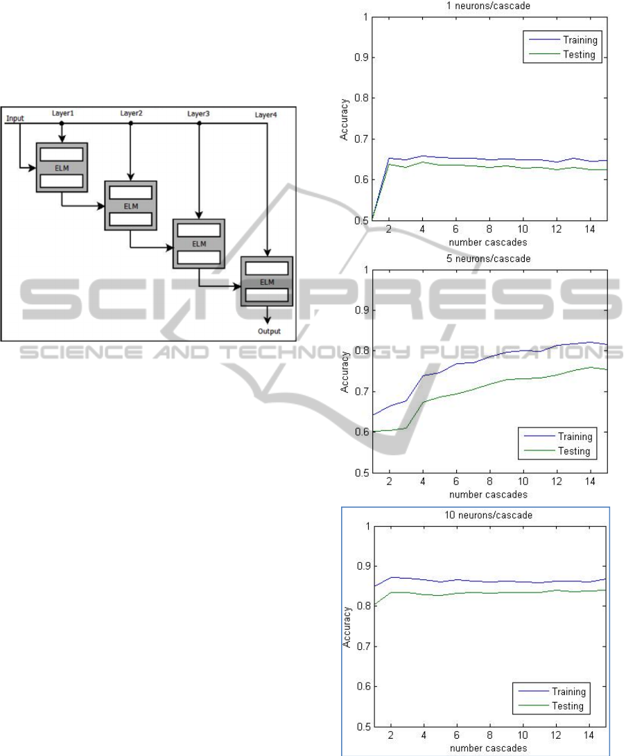
Figure 6: Schematic of single cascade ELM.
The main feature of this algorithm is the feeding
of the previous cascade into the trained layer of the
next cascade rather than into the random layer. This
is important because if the cascade is fed into the
random layer any correlation learnt in the previous
cascade will be lost again. On the other hand the
input data needs to go through the random layer
before it can be used for training.
Figure 7 shows the results for numbers of
neurons in each cascade, for 1, 5, and 10 hidden
neurons each. As expected the Test results are
always a bit less than the Training results.
Our results show that the ability of the network
to learn improves slightly as cascades are added but
generally only for the first few cascades. The
number of neurons in each cascade has a more
significant effect on its learning capacity.
There is a straightforward possible explanation,
when the topology of the network is considered in
more detail. Clearly the amount of information
which can be stored in each cascade is limited by the
number of neurons in the output layer. If only the
previous layer contributes to the next cascade then
as cascades are added the network rapidly reaches its
full learning capacity. When there are many
cascades then earlier cascades will have little or no
effect on the result.
Figure 7: Single Cascade results for 2 spirals dataset.
3.4 Full Cascade
An extension to our single cascade is to provide the
outputs of all previous cascades to the trained layers
ExtremeLearningMachineswithSimpleCascades
275
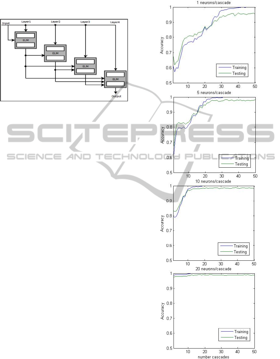
of subsequent cascades. We call this a full cascade
extreme learning machine, see Figure 8.
Figure 8: Schematic of full cascade ELM.
In Figure 9 we show the results for different
numbers of hidden neurons in each cascade neurons.
In each of the first three results shown, for 1, 5, 10
neurons per cascade, the testing curve is initially
higher than the training curve before crossing over.
The final graph showing the results for 20 neurons
has the training results always above the testing
results.
These results are substantially improved over the
simple cascade results shown earlier in in Section
3.3, Figure 7.
Our results show that even with only 1 neuron in
each cascade the network is capable of reaching
95% accuracy with test data. As expected, the more
neurons in each cascade the less cascades are
required to reach a high degree of accuracy.
3.5 Trade-offs: Accuracy, Neurons per
Cascades and Number of Cascades
Full cascade ELM training times are longer than
simple ELM but not excessively so. To train a
network with 5 neurons per cascade and 30 cascades
took 0.078 seconds on the experimental machine this
compares to .02 seconds for a simple ELM machine
with 40 neurons in the hidden layer. This is a ratio of
3.9 for time, and 3.75 for number of neurons, so the
cascade structure added roughly 4% runtime. Our
results were similar for the diabetes dataset.
Figure 10 demonstrates the relationship of
neurons/cascade, number of cascades and accuracy
in a single surface plot. The shape of the surface
along the two axis shows:
(x) a pure ELM as the number of neurons in the
hidden layer increases, and
(y) a pure cascade machine with one neuron in
each hidden layer.
Figure 9: Full Cascade results for 2 spirals dataset.
SIMULTECH2015-5thInternationalConferenceonSimulationandModelingMethodologies,Technologiesand
Applications
276
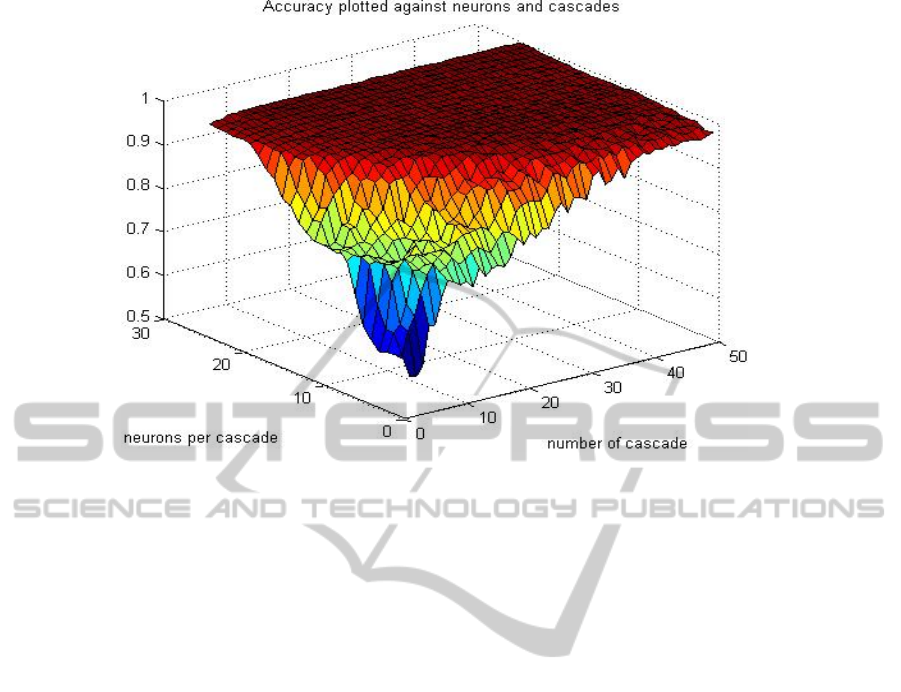
Figure 10: Full Cascade trade-offs: accuracy, cascade size and number.
4 CONCLUSIONS AND FUTURE
WORK
We have introduced 3 simple cascades into extreme
learning machines. Our shallow cascade was
surprisingly effective when the number of neurons in
ELM layers were small. Our simple cascade
architecture worked but provided little benefit. Our
full cascade ELM architecture was able to achieve
high performance even with a single neuron per
ELM cascade, is indicative of some generality of our
approach.
Our future work will include significantly more
datasets to extend our results beyond being
indicative, the analysis of network structure to
improve performance (Gedeon, 1997), un-freezing
some weights and training briefly using RPROP
(Treadgold and Gedeon, 1997), and the use of noise
to improve network performance (Brown et al.,
2004).
ACKNOWLEDGEMENTS
We thank the four referees for their constructive
comments, and have included as many of them as
we could. The rest will inform our future work.
REFERENCES
Bartlett, P. L. (1998). The sample complexity of pattern
classification with neural networks: the size of the
weights is more important than the size of the
network. Information Theory, IEEE Transactions on,
44(2), 525-536.
Bin, L., Yibin, L., & Xuewen, R. (2011). Comparison of
echo state network and extreme learning machine on
nonlinear prediction. Journal of Computational
Information Systems, 7(6), 1863-1870.
Blake, C., & Merz, C. J. (1998). UCI Repository of
machine learning databases. Accessed August 2014.
tinyurl.com/Diebates.
Brown, W. M., Gedeon, T. D., & Groves, D. I. (2003).
Use of noise to augment training data: a neural
network method of mineral–potential mapping in
regions of limited known deposit examples. Natural
Resources Research, 12(2), 141-152.
Fahlman, S. E. and C. Lebiere, "The cascade-correlation
learning architecture," Advances in Neural
Information Processing, vol. 2, D.S. Touretzky, (Ed.)
San Mateo, CA:Morgan Kauffman, 1990, pp. 524-532.
Gedeon, T. D. (1997). Data mining of inputs: analysing
magnitude and functional measures. International
Journal of Neural Systems, 8(02), 209-218.
Gedeon, T. D., & Kóczy, L. T. (1998, October).
Hierarchical co-occurrence relations. In Systems, Man,
and Cybernetics, 1998. 1998 IEEE International
Conference on (Vol. 3, pp. 2750-2755). IEEE.
Huang, G. B., Wang, D. H., & Lan, Y. (2011). Extreme
learning machines: a survey. International Journal of
Machine Learning and Cybernetics, 2(2), 107-122.
ExtremeLearningMachineswithSimpleCascades
277

Huang, G. B., Zhu, Q. Y., & Siew, C. K. (2004, July).
Extreme learning machine: a new learning scheme of
feedforward neural networks. In Neural Networks,
2004. Proceedings. 2004 IEEE International Joint
Conference on (Vol. 2, pp. 985-990). IEEE.
Jaeger, H. (2001). The “echo state” approach to analysing
and training recurrent neural networks-with an
erratum note. Bonn, Germany: German National
Research Center for Information Technology, GMD
Technical Report, 148, 34.
Kools, J. (2013). 6 functions for generating artificial
datasets. Accessed August 2014. www.mathworks.
com.au/matlabcentral/fileexchange/41459-6-
functions-for-generating-artificial-datasets.
Marques, I., & Graña, M. (2012). Face recognition with
lattice independent component analysis and extreme
learning machines. Soft Comput., 16(9):1525-1537.
Rho, Y. J., & Gedeon, T. D. (2000). Academic articles on
the web: reading patterns and formats. Int. Journal of
Human-Computer Interaction, 12(2), 219-240.
Riedmiller, M. (1994). Rprop - Description and
Implementation Details, Technical Report, University
of Karlsruhe.
Rumelhart, D. E., Hinton, G. E., & Williams, R. J.,
“Learning internal representations by error
propagation,” in Rumelhart, D. E., McClelland, J.,
Parallel distributed processing, v:1, MIT Press, 1986.
Shen, T., & Zhu, D. (2012, June). Layered_CasPer:
Layered cascade artificial neural networks. In Neural
Networks (IJCNN), The 2012 International Joint
Conference on (pp. 1-7). IEEE.
Sun, Y., Yuan, Y., & Wang, G. (2014). Extreme learning
machine for classification over uncertain data.
Neurocomputing, 128, 500-506.
Tissera, M. D., & McDonnell, M. D. (2015). Deep
Extreme Learning Machines for Classification. In
Proceedings of ELM-2014 Volume 1 (pp. 345-354).
Springer International Publishing.
Treadgold, N. K., & Gedeon, T. D. (1997). A cascade
network algorithm employing progressive RPROP. In
Biological and Artificial Computation: From
Neuroscience to Technology (pp. 733-742). Springer
Berlin Heidelberg.
Wefky, A., Espinosa, F., Leferink, F., Gardel, A., & Vogt-
Ardatjew, R. (2013). On-road magnetic emissions
prediction of electric cars in terms of driving dynamics
using neural networks. Progress In Electromagnetics
Research, 139, 671-687.
Wong, P. M., Taggart, I. J., & Gedeon, T. D. (1995). Use
of Neural-Network Methods to Predict Porosity and
Permeability of a Petroleum Reservoir. AI
Applications, 9(2), 27-37.
SIMULTECH2015-5thInternationalConferenceonSimulationandModelingMethodologies,Technologiesand
Applications
278
