
Taguchi Method or Compromise Programming as Robust Design
Optimization Tool: The Case of a Flexible Manufacturing System
Wa-Muzemba Anselm Tshibangu
Morgan State University, Department of Industrial and Systems Engineering,
1701 E Cold Spring Lane, Baltimore, MD 21251, U.S.A.
Keywords: Robust Design, Optimization, Taguchi Method, Compromise Programming, Fms, Simulation.
Abstract: Competitive advantage of a firm is usually reflected through its superiority in production resources and
performance outcomes. In order to achieve high performance (e.g., productivity) and significantly improve
product quality, major US industries have promoted and implemented Robust Design (RD) techniques
during the last decade. RD is a cost-effective procedure for determining the optimal settings of the control
factors that make the product performance insensitive to the influence of noise factors. In this research, we
employ and compare two RD optimum-seeking methods to optimize a flexible manufacturing system
(FMS). Taguchi Method (TM), which uses robust design concept, i.e., Signal-To-Noise Ratio (S/N) to
reduce the output variation, is applied first. Taguchi’s approach to robust design drawn much criticism
because it relies on the signal-to-noise (S/N) ratio for the optimization procedure. Because of this paramount
criticism, a second method known as the Compromise Programming (CP) approach, i.e., the weighted
Tchebycheff, is also used. This method formulates the robust design as a bi-objective robust design (BORD)
problem by taking into account the two aspects of the RD problem, i.e. minimize the variation and optimize
the mean. This approach seeks to determine the RD solution which is guaranteed to belong to the set of
efficient solutions (Pareto points). Both methods use a RD formulation to determine an optimal and robust
configuration of the system under study. The results gained through simulations and analytical formulations
show that the current ways of handling the multiple aspects of the RD problem by using Taguchi’s S/N ratio
may not be adequate.
1 INTRODUCTION
A variety of approaches has been proposed for the
design, control and optimization of manufacturing
systems in order to find the best parameter settings
for an optimal operation. These techniques include
mathematical programming, queuing networks,
computer simulation, Artificial Intelligence (AI). It
has been noticed that the usefulness of any of these
tools depends on the nature of the problem.
Computer-aided and automated production and
manufacturing systems can be described or
characterized as a group of processing centers
connected by an automated material handling system
under computer control. Selecting the optimal
setting in such an environment is critically important
since it affects the manufacturing performance
measures, production cost and the loss due to a plant
performance deviation from the company-identified
target value. The selection of the appropriate setting
of input factors in order to attain the required
process target (mean) is of major interest in various
manufacturing optimization models including
Robust Design models. Material handling system is
the back-bone of a Flexible Manufacturing System
(FMS). It connects various production functions and
regulates movement of parts through the facility.
Automated guided vehicles (AGVs) have been the
most popular choice among the several types of
material handlers available and used in FMSs.
Achievement of high performance from an
Automated Guided Vehicle System (AGVS) is
influenced by several “Design” and “Operational
Control" issues. These include specifying the type
and number of vehicles to be employed, specifying
appropriate guide path configuration together with
locating load transfer stations, locating vehicle
buffering areas and specifying their loading
capacity, specifying vehicle dispatching and routing
strategies, managing traffic, specifying unit load
sizes, specifying central and/or local work-in-
485
Tshibangu W..
Taguchi Method or Compromise Programming as Robust Design Optimization Tool: The Case of a Flexible Manufacturing System.
DOI: 10.5220/0005547404850492
In Proceedings of the 12th International Conference on Informatics in Control, Automation and Robotics (ICINCO-2015), pages 485-492
ISBN: 978-989-758-123-6
Copyright
c
2015 SCITEPRESS (Science and Technology Publications, Lda.)

process storage capacity, specifying the machine
queue discipline, etc.
2 OPTIMIZATION OF FMSS
Most of the contemporary manufacturing firms,
typically flexible manufacturing systems possess a
certain randomness that invites complexity. As the
degree of complexity increases, it becomes difficult
if not impossible to use analytical models to study
the manufacturing system behaviors. Therefore,
simulation is widely used to study manufacturing
systems’ performances (Tshibangu, 2004). But,
although a significant amount of simulation studies
has been conducted for design and analysis of FMSs,
especially to construct performance models, this
technique does not provide optimal solutions.
The present study analyzes an hypothetical Flexible
Manufacturing System and aims to maximize the
Throughput Rate (TR) of such a system while
making the system robust, i.e., insensitive to
uncontrollable factors otherwise known as noise. To
achieve this, the research uses the well-known
Robust Design (RD) methodology. Typically, when
implemented by optimization, robust design is
achieved by optimizing the mean of performance
and minimizing the variation of performance.
3 APPROACH IN THIS STUDY
This study employs one of the well-known robust
design methodologies, namely the Taguchi Method
(TM), to find the optimal combination of input
factor settings (levels) that would optimize (i.e.,
maximize) the throughput rate (TR) of the selected
hypothetical Flexible Manufacturing System. In
particular, the research uses the two-part orthogonal
array for experimental design and the signal-to-
noise-ratio (S/N-ratio) as the robust optimization
criterion.
Although Taguchi’s Methods (TM) are widely
accepted in the industry, and although the inclusion
of noise factors for the purpose of design
optimization has been considered as an innovative
concept by several researchers, others have severely
criticized its statistical methods. Taguchi’s approach
to robust design has particularly drawn a high
amount of criticism because it relies on the signal-
to-noise (S/N) ratio for the optimization procedure
(Pignatiello and Ramberg, 1991; Tshibangu, 2004).
Because of the various criticisms formulated in
disfavor of using the signal-to-noise ratio as
optimization criterion following Taguchi robust
design approach, this research paper has decided to
address the multiple aspects of the robust design
problem by exploring a different approach known as
the Compromise Programming (CP), specifically the
Tchebycheff method. Compromise Programming
(CP) was first proposed by Zeleny (1974) and
subsequently used by many researchers (Randhir,
2000, Gorantiwar et. al., 2010, Gharis, 2012).
CP identifies the best compromise solution as the
one that has the shortest distance to an ideal point
where the multiple objectives/responses as
formulated in the optimization objective function
problem simultaneously reach their optimal values.
The ideal point is not practically achievable but may
subsequently be used as a base point or target.
This study uses “Simulation” as an approach to
modeling an hypothetical FMS and applies the two
above mentioned methods, namely TM and CP
separately while using the Throughput Rate (TR) as
the unique and single performance measure. The
results of both methods are subsequently compared
before drawing conclusions in terms of advantages
and disadvantages of one method over another. The
paper focuses on the determination of the best
combination of design- and operational-related
parameters to optimize the hypothetical FMS with
respect to the throughput rate (TR). The reason
being that a high TR would result into the realization
of a higher productivity, under the assumption that
the use of specific queue discipline rules such as
FIFO (First-In-first-Out) or Shortest Processing
Time (SPT) would generally yield a lower Mean-
Flow-Time (MFT) as demonstrated by several
researchers (Shang, 1995; Tshibangu, 2004, 2013)
4 TAGUCHI ROBUST DESIGN
RD is a cost effective methodology for determining
the optimal setting of the control factors that would
make the product performance insensitive to the
influence of noise factors (Cho et al., 2000). Taguchi
proposed a three-step approach to product and
process design. These are system design, parameter
design, and tolerance design. In this study, the
philosophy and experimental design principles
developed by Taguchi (1986) will be applied.
The reader is referred to Taguchi (1986),
Pignatiello et. al. (1991), Tshibangu (2004, 2013)
for details about Taguchi Method and RD
implementation steps. The main advantage of using
ICINCO2015-12thInternationalConferenceonInformaticsinControl,AutomationandRobotics
486

Taguchi Method (TM) is that products and processes
become robust to uncertain conditions.
The common meaning of “robust” is that product
functions are insensitive to variations in real
application environment. Taguchi (1985) first
suggested the use of the so-called orthogonal arrays
using inner array for control factors and an outer
array for the uncontrollable (noise) factors and
Signal-To-Noise (S/N) ratios as optimization tool.
4.1 Orthogonal Array
The goal of this research is to study the effects of the
noise factors on the performance criterion and
optimize such effects. Thus, designs that enable this
research to study these effects in an economical way
must be favored. Consequently, it is logical to
choose the orthogonal arrays or fractional factorial
designs that allow to study the effects of noise
factors as well as the interaction effects by running
the minimum (economical) number of experiments.
The matrix that designates the settings of
controllable factors for each run is called inner array.
The matrix that designates the setting of
uncontrollable factors is called an outer array.
The nomenclature of the orthogonal array is
)(
b
a
XL
, where “
X
” represents the number of
levels to be explored, “
a ”represents the number of
experimental runs and “
b
” represents the number of
factors that are studied. After the appropriate designs
for both control and noise factors are chosen, they
are assigned to the inner and outer arrays,
respectively. The inner-outer array design is the
main strategy for robust design. The noise factors
are assigned to the outer array to find some level of a
control factor that does not result in much variation
in spite of noise factors definitely being present.
4.2 Signal-to-Noise Ratio (S/N)
An adequate performance measure should
incorporate both the desirable and the undesirable
aspects of the output characteristics. A metric
developed by Taguchi in order to optimize a design
is the Signal-to-Noise ratio (S/N) using the ratio of
the variation in output response resulting from
control factors to that resulting from unpredictable
or noise factors. In the Taguchi method, the term
signal represents the desirable component. The term
noise represents the undesirable component and is a
measure of the variability of the output
characteristic, which preferably should be as small
as possible. The Signal-to-Noise Ratio is defined as:
)log(10/ MSDNS −=
(1)
The Mean Squared Deviation
)(MSD
is defined for
different quality characteristics. For Smaller-The-
Better (STB):
nyyyyMSD
n
/)...(
22
3
2
2
2
1
++++=
(2)
For Nominal-The-Best (NTB):
nTy
TyTyTyMSD
n
/)...(
)()()(
2
2
3
2
2
2
1
−+
−+−+−=
(3)
For Bigger-The-Better (BTB):
nyyyyMSD
n
/)1...111(
22
3
2
2
2
1
+++=
(4)
where
y
i
=The results of experiments in each row
T = Target value of results
n = Number of noise combinations
4.3 Quality Loss Function (QLF)
Taguchi also uses the Quality Loss Function (QLF)
as a metric for robust optimization. The main idea is
that a loss is always incurred when a product/process
performance deviates from its target value,
regardless of how small the deviation is. The QLF is
given by:
2
)()( TYKYL −= (5)
where
K
is the (positive) loss function coefficient,
Y
is the random variable of quality characteristic
y
,
T
is the target or desired value of the quality
characteristic of interest.
The reader is referred to the extensive
discussions in the literature on various Loss
Functions (Berger 1985, Pignatiello 1991). An
interesting and desirable characteristic of the QLF is
that it was proven (Ribeiro 1995, Tshibangu 2004,
2013): that for the Nominal-the- Better (NTB) type
problem, the expected loss is given by:
])([)],([
22
μσ
−+= TKTYLE
(6)
where
σ
and
2
σ
represent the mean and variance
of
Y
, respectively. It is interesting to note that
minimizing the quality loss can be achieved by
minimizing both the variance
)(
2
σ
and the bias
)( T−
μ
or difference between the mean and the
target
)(
μ
−T
.
Chen et al. (1998) found that one issue that has
not been adequately addressed in the previous
investigations is the multiple aspects of the objective
in robust design. They suggest for the robust design
problem a formulation that would consider
TaguchiMethodorCompromiseProgrammingasRobustDesignOptimizationTool:TheCaseofaFlexibleManufacturing
System
487

“optimizing the performance” and “minimizing the
variance” as two objective functions to be optimized
separately. Their approach is used in the present
study.
Therefore, to address the multiple aspects of
robust design, it is necessary to treat it as a multi-
objective optimization problem. Since the
performance variation is often minimized at the cost
of scarifying the best performance, a tradeoff
between the aforementioned aspects should
necessarily take place. There are several ways of
dealing with the tradeoff between multiple
objectives. Chen et al. (1998) used a combination of
the rigorous multi-objective mathematical
programming method and the principles of decision
analysis to address the multiple aspects of the
objective in robust design.
They proposed the use of Compromise
Programming approach (CP), i.e., the Tchebycheff
method in place of the traditional WS method. For
details on the Compromise Programming (CP)
method, the reader is referred to Park et. al. (2001).
5 COMPROMISE
PROGRAMMING
The CP was developed by Zeleny (1974), under the
motivation of looking for a more powerful method
in generating a Pareto set.
Let
[]
)(),...,()(
1
xfxfxF
m
=
and
mixf
i
,...,1),( =
,
be real-valued continuous functions defined in
m
R
.
Let X denotes the design space that is formed by
both the design constraints and the range of design
variables x, and
m
RxFY ⊂= )( be the objective
space, in a multi-objective problem formulated as:
minimize
)( xF
subject to
m
RXx ⊂∈
(7)
A point
0
x
is called a Pareto solution of the multi-
objective optimization problem if there is no other
feasible point
x
, such that )()(
0
xfxf
ii
≤ ,
mi ,...,1=
, with strict inequality for at least one
index
i . The image )(
0
xF ) of a Pareto solution in
the objective space is called the efficient solution.
The common practice for finding Pareto
solutions has been the Weighted Sum (WS) method
that performs the minimization of a linear
combination of the objective functions. The
corresponding weighted-sum problem
()
)( wWSP
is:
minimize
=
m
i
ii
xfw
1
)(
subject to
m
RXx ⊂∈ (8)
where
miw
i
,...,1,0 =≥ and
1
1
=
=i
i
w
Scalars
i
w are referred to as the weights assigned to
the objective
mif
i
,...,1, = , and determine the
importance of each objective. It is well recognized in
the literature that an optimal solution of the
()()
)(wWSP
for any positive weights is always a
Pareto solution of the original problem, which
consists of minimizing each objective function
individually over the design space (Gorantiwar et.
al. 2010, Anita et. al., 2012, Gharis 2012).
The basic idea of the CP method is to identify an
ideal solution (utopia point) where each attribute
under consideration achieves its optimum value. In
the case of conflict among the different attributes,
the designer seeks a solution, which is the closest
possible to the ideal solution. In Chen et al.1998, the
authors review and compare two approaches to
finding its Pareto set: the WS approach and the CP
method. They show the limitations of the former and
the advantages of the latter. Typically, the
advantages of the
),( wCP ∞
approach over the
WS method in locating the efficient multi-objective
robust design solutions (Pareto points) are
illustrated. The
),( wCP ∞
also known as the
weighted Tchebycheff approach is very useful in
generating Pareto solutions.
In this paper, beside the Taguchi’s approach
(TM), the Compromise Programming
),( wCP ∞
which guarantees that all efficient solutions of the
problem are generated, is also used to solve a bi-
objective robust design problem (BORD). The
results of both methods are further analyzed and
compared.
6 ROBUST DESIGN USING CP
Based on the principles of the CP approach, a robust
design procedure has been proposed by Chen et al.
1998 to address the multiple aspects of robust
design. The first step is to transform the traditional
optimization problem into a RD formulation, that is,
an engineering design problem is stated using the
conventional optimization model as follows:
minimize
)(xf
)
ICINCO2015-12thInternationalConferenceonInformaticsinControl,AutomationandRobotics
488

subject to
,0)( ≤xg
j
Jj ,...,2,1=
UL
xxx ≤≤ (9)
where
x
,
L
x and
U
x are vectors of design variables,
their lower bounds and upper bounds, respectively;
)(xf
is the objective function and
)(xg
j
is
the
thj −
constraint function. The RD design
model can therefore be stated as a bi-objective
robust design (BORD) problem as follows (Gharis,
2012):
minimize
[
]
ff
σμ
,
subject to
0)(
1
≤Δ
∂
∂
+
=
i
m
i
i
j
jj
x
x
g
kxg
,
Jj ,...,2,1=
xxxx
UxL
Δ−≤≤Δ+ (10)
where
f
μ
and
f
σ
are the mean and standard
deviation of the researched objective function,
)(xf
respectively.
The next step once the problem is transformed
into a BORD is to seek for the ideal solution (utopia
point) by optimizing
f
μ
and
f
σ
individually, using
the model as stated in Equation (9).
f
μ
can be
optimized by using either the “Smaller-the-Better”,
the “Nominal-the-Best” and the “Larger-the-Better”.
But it is always desired to minimize
f
σ
. The utopia
point found through the abovementioned process is
denoted
[
]
**
,
ff
σμ
.
Knowing the ideal solution of the robust design
problem, the designer needs to specify a preference
structure by assigning weights
1
w and
2
w to
represent the relative importance of the two
objectives. The process stops only when a
satisfactory solution is reached. Details on technique
relating utility function optimization to CP is
extensively provided in Chen et al. 1998.
7 EXPERIMENTS +
METHODOLOGY
The steps used for the robust design methodology
applied in this study can be summarized as follows:
1) Choose the levels of the control factors and
noise factors.
2) Chose the appropriate design for both control
and noise factors.
3) Assign the control factor to the inner array and
noise factor to the outer array.
4) Conduct the experiments using discrete-event
simulation program (ARENA is used in this
study).
5) Calculate the mean and the variance of the
Throughput Rate (TR).
6) Apply Taguchi’s Robust Design method to
optimize the throughput mean and minimize
the variation in the Throughput Rate, and
predict the control factors that optimize the
manufacturing system under study.
7) Apply the CP approach to Robust Design for
the same purpose as in 6.
8) Apply confirmation methods such as residual
analysis.
9) Run the confirmatory experiments for each case
(i.e., Taguchi and CP).
10) Compare results and make final conclusions.
7.1 Shop Conditions and Simulation
Model
The manufacturing system analyzed in this research
is composed of 5 workstations, one loading and one
unloading station, as illustrated in Tshibangu (2003).
Each workstation is constituted of one machine. The
control factors explored in this research are the
number of AGVs, the number of pallets, the buffer
size per machine, the machine dispatching rule, the
AGV dispatching rule, the interarrival time and the
AGV speed. Uncontrollable factors considered are
the MTBF (Mean Time Between Failure) and
MTTR (Mean Time To Repair). Taguchi
experimental design principles and simulation were
used to measure the Throughput Rate, the single
performance measure criterion considered in the
present study. Table 1 gives the factors and their
associated levels for the simulation of the FMS
under study.
Consider a system involving a response
Y
(i.e.,
throughput) which depends on the level of
k
control
factors
),...,,(
21 k
xxx . Suppose that m replicates
are taken at each of the design points.
Finding the true functional relationship between
the dependent variable
Y
(Throughput Rate) and the
independent variables
k
x will lead, when using
regression analysis, to an approximating function of
the form:
ii
k
xY
ββ
+=
1
0
(11)
TaguchiMethodorCompromiseProgrammingasRobustDesignOptimizationTool:TheCaseofaFlexibleManufacturing
System
489
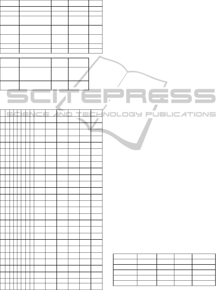
Table 1: Factors and their levels for simulation.
Designation Controllable Factors Level 1 Level 2 Level 3
X
1
Number of AGVs 2 5 8
X
2
Number of Pallets 80 90 100
X
3
Buffer Size per
Machine
4 8 12
X
4
Machine
Dispatching Rule
TPT SPT.TOT SPT
X
5
AGV Dispatching
Rule
FCFS STD LQS
X
6
Interarrival Time 30 min. 20 10
X
7
AGV Speed 60 f/min 80 100
Uncontrollable
Factors
Level 1 Level 2
X
8
Mean Time
Between Failure
(MTBF)
300 (Low) 700 (High)
X
9
Mean Time to
Repair (MTTR)
50 (Low) 90 (High)
Table 2: Parameter design results.
Inner Array Outer Array Response
n A B C D E F G H1 I1 H1 I2 H2 I1 H2 I2 Y S/N
1 1 1 1 1 1 1 1 149 133 233 161 169 44.018
2 2 2 1 1 2 2 2 194 140 348 241 230.75 45.889
3 3 3 1 1 3 3 3 279 145 352 242 254.5 46.698
4 2 2 1 2 1 3 3 224 121 399 232 244 45.486
5 3 3 1 2 2 1 1 219 121 369 293 250.5 45.681
6 1 1 1 2 3 2 2 276 207 373 268 281 48.418
7 3 3 1 3 1 2 2 241 187 385 303 279 47.996
8 1 1 1 3 2 3 3 257 195 328 272 263 47.942
9 2 2 1 3 3 1 1 285 215 361 265 281.5 48.55
10 2 3 2 1 1 2 3 318 217 416 305 314 49.24
11 3 1 2 1 2 3 1 240 169 385 255 262.25 47.299
12 1 2 2 1 3 1 2 202 193 265 212 218 46.583
13 3 1 2 2 1 1 2 184 141 375 244 236 45.861
14 1 2 2 2 2 2 3 251 218 352 263 271 48.28
15 2 3 2 2 3 3 1 298 198 415 274 296.25 48.547
16 1 2 2 3 1 3 1 233 190 281 231 233.75 47.126
17 2 3 2 3 2 1 2 269 212 354 241 269 48.148
18 3 1 2 3 3 2 3 376 223 415 346 340 49.857
19 3 2 3 1 1 3 2 353 268 380 328 332.25 50.204
20 1 3 3 1 2 1 3 236 149 316 220 230.25 46.304
21 2 1 3 1 3 2 1 247 196 371 283 274.25 48.085
22 1 3 3 2 1 2 1 243 157 326 207 233.25 46.466
23 2 1 3 2 2 3 2 309 263 389 328 322.25 49.91
24 3 2 3 2 3 1 3 271 220 416 289 299 48.858
25 2 1 3 3 1 1 3 258 214 346 265 270.75 48.279
26 3 2 3 3 2 2 1 241 219 396 318 293.5 48.67
27 1 3 3 3 3 3 2 267 206 377 298 284 48.547
If there is a curvature in the system, then a
polynomial of higher degree must be used, such as
the second-order model:
+++=
ij
jiiji
k
ii
k
ii
xxxxY
ββββ
11
0
(12)
Equations 11 and 12 will be used in the CP
approach. The Taguchi Method experimental design
as carried out in this study results into 27 design
configurations to be run using simulation package
ARENA
TM
. The coded experimental results for the
27 runs under the four uncontrollable factor
combination levels are given in Table 2.
7.2 Taguchi Method Results an
Analysis
For the Taguchi approach, analysis of data will first
involve calculation of
Y
and the
NS /
ratio. In
this research, Throughput Rate has the “Bigger-the-
Better” characteristic, because it desired to be
maximized. Therefore, Equation 4 has to be used for
the
NS /
calculations.
The ANOVA (not represented here) for the
regression model including all the variables has
confirmed what is already known from previous
studies (Tshibangu, 2003), namely that the number
of pallets is not a significant factor. Although AGV
and machine dispatching rules have shown a slight
significance, they are considered as insignificant
factors in this study. Therefore, the number of AGVs
(X
a
), the buffer size (X
b
), the interarrival time (X
c
)
and the speed of AGV (X
d
) as renamed variables will
be considered as the only factors of interest in this
study. The confidence interval level used in this
study is 95%. After analyzing the main and
interaction effect plots as suggested by Taguchi, the
factors (and their levels) recommended by the
Taguchi Method and confirming the regression
analysis conclusions, study are found to be : X
a
= 5 ,
X
b
= 12, X
c
= 20, and X
d
= 80, leading to a maximum
throughput of 253 units in coded data. Table 3
displays the regression analysis coefficients.
Table 3: Regression analysis coefficient and R
2
.
Predictor Coeff. StDev T p
Constant -36.667 6.023 -6.09 0.000
AGV 7.667 1.475 5.20 0.000
Buffer 6.35 1.475 4.32 0.000
InterArr 6.333 1.475 4.29 0.000
SpeedAgv 5.667 1.475 3.84 0.001
S = 6.260 R-Sq = 78.1% R-Sq(adj) = 74.2%
ICINCO2015-12thInternationalConferenceonInformaticsinControl,AutomationandRobotics
490
A first-order model to these data by least squares
gives, for the best subset, in coded variables the
following equation:
Y
ˆ
= 7.67 AGV + 6.33 Buffer + 6.33 InterArr + 5.67
SpeedAgv - 36.7 (13)
Using now X
a
, X
b
, X
c
, and X
d
for number of AGVs,
Buffer size, Interrarrival time and AGV speed,
respectively, Equation 13 is written as follows:
Y
ˆ
= 7.67 X
a
+ 6.35 X
b
+ 6.33 X
c
+ 5.67 X
d
- 36.7 (14)
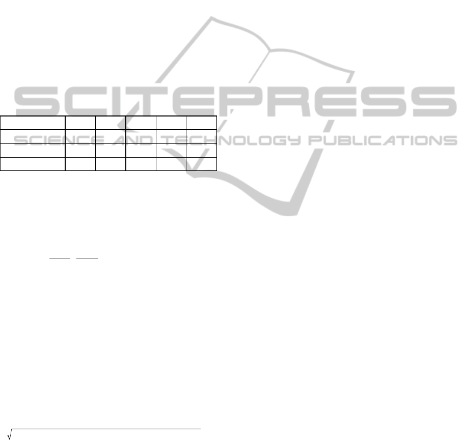
The ANOVA Table for the model is displayed in
Table 4. It shows all the four factors significant as
confirmed by the F-test results for the overall
regression and the regression coefficients. All the
interactions between factors are considered to be
insignificant.
Table 4: ANOVA Best subsets regression model.
Source DF SS MS F p
Regression 4 3080 770 19.65 0.0
Residual Error 22 862 39.18
Total 26 3942
7.3 CP Method Results and Analysis
The BORD problem for the FMS configuration
under study is formulated as follows:
Minimize
∗∗
f
f
f
f
σ
σ
μ
μ
,
Subject to 2 + Δ X
1
≤ X
1
≤ 8 - Δ X
1
4 + Δ X
2
≤ X
2
≤ 12 -Δ X
2
-30 +Δ X
3
≤ X
3
≤ -10-Δ X
3
60 + Δ X
4
≤ X
4
≤ 80 -Δ X
4
(15)
where the mean function and standard deviation can
be derived from the following equations:
f
μ
= E[Y(x
i
)] = 7.67 E[X
a
] + 6.35 E[X
b
] +
6.33 E[Xc] +5.67 E[X
d
] –36.7 (16)
))(((
if
xYVar=
σ
(17)
=
)(67.5)(33.6)(35.6)(67.7
4
2
3
2
2
2
1
2
XVarXVarXVarXVar +++
It worth it to note that if the function was non-linear,
the mean function and the standard deviation could
have been derived using first-order Taylor expansion
series. To seek the ideal solutions,
*
f
μ
,
*
f
σ
, the
above optimization problem formulated in (17) is
solved separately as the design objective. Note that
in Equation (15), in order to study the variation of
the constraints, the original constraints are modified
by adding a penalty term to each of them. The
penalty factors are to be determined by the designer.
The bounds of design variable vector
()
x are also
modified to ensure feasibility under deviation. When
the size of the variation is considered as Δ X = 0
(ΔX
a
= Δ X
b
= Δ X
c
= Δ X
4
= 0) and, and the penalty
factor
k
is taken as 1.0 (in this example (
0=
j
g
,
the ideal solution under the assumption of equal
density functions, are obtained in coded values, as
)2.79,8.19,92.7,95.4(
*
f
X
μ
for
258
*
=
f
μ
units, and
)2.88,0.22,0.4,0.2(
*
f
X
σ
for
22.109
*
=
f
σ
.
8 CONCLUSIONS
The primary objective of this paper is to propose an
enhanced optimization strategy by formulating the
robust design procedure using the recent
development on mathematical programming
methods and decision analysis principles. The
multiple aspects of the objective in RD are
addressed explicitly and designers are allowed to
select their preferred structure among a set of
candidate optimal solutions.
The study presents two methods for FMS design
and optimization, particularly for AGVs and
machines (work stations). Because it is almost
impossible to predict the response (Throughput Rate
in this case) as mathematical functions of the factors,
an empirical (simulation) approach has been
adopted.
First, Taguchi Method is used to act as a
screening process and to quickly identify the optimal
area. This is important, because no more
experimental effort has to be spent on the non-
significant factors, and the designer can quickly
concentrate on the important (significant) factors
that have been identified. Taguchi Method also helps
to reduce the noise factors rather than eliminating
them (which is neither practical nor feasible).
Furthermore, Taguchi Method provides a unique
fashion for optimization when qualitative factors are
concerned.
Because there is still some controversy about
optimization tools used by Taguchi Method such as
orthogonal arrays, signal-to-noise ratios, and linear
TaguchiMethodorCompromiseProgrammingasRobustDesignOptimizationTool:TheCaseofaFlexibleManufacturing
System
491

graphs, a second optimization approach known as
the Compromise Programming is proposed and
applied. The basic idea of CP is to identify an ideal
solution (utopia point) where each attribute under
consideration achieves its optimum value (Adeyeye
et. al., 2010,
Anita et. al. , 2012).
This enhanced optimization model in robust
design considers both the product/process bias and
the variance. It was numerically demonstrated that
this proposed model might provide a better solution
in terms of control factor settings in an FMS or other
environments. Many of the previous studies have
concentrated on the minimization of the variance
while keeping the bias at zero. But, it has been
shown (Cho et al, 2000) that there are situations
where the minimum variance with a zero bias may
not provide the minimum expected loss.
When compared to the existing methods for
robust optimization such as Taguchi’s S/N ratio, the
proposed approach has many advantages (Chen et
al. 1998), namely: capability of generating the
efficient solutions, interactive robust design
procedure, significance of the multi-objective
approach to robust design, etc. As a research
strategy however, we suggest that these two methods
be used together, especially when there are
qualitative factors involved. We propose that the
region of investigation be determined by the TM
before using CP. When TM is used alone, the
interaction factors cannot be fully taken into account
due to the limit of the linear graph in the orthogonal
array.
On one hand, the optimization is only done over
the points (three levels in this study) considered in
the design. These points (factor levels) may not lead
the true optimum when continuous variable are
involved. On the other hand the CP approach is
unable to handle qualitative variables. Using the two
methods combined will help designers to determine
what level of the input factors and AGV and
machine dispatching rules will maximize the
Throughput Rate for a specific FMS. Simulation,
Taguchi and CP approaches to RD are powerful
tools to improve the design and performance in the
FMS environment. Further research may consider
multiple performances measures instead of one used
in this study.
REFERENCES
Adeyeye et. al., 2012. Multi-objective methods for
welding flux performance Optimization, RMZ –
Materials and Geoenvironment, Vol. 57, No. 2, pp.
251-270.
Anita et. al. 2012, A Mathematical Analysis of
Compromising Programming Techniques. IOSR
Journal of Mathematics ISSN: 2278-5728. Vol. 3.
Berger, J.O., 1985,.Statistical Decision Theory and
Bayesian Analysis (New York: Springer-Verlag).
Chen, W., Wiecek, M.M., Zhang, J., 1998, Quality Utility-
A Compromise Programming Approach to Robust
Design, ASME Design Technical Conference, paper
no. DAC5601, Atlanta, GA.
Cho, B.-R, Kim, Y.J., Kimbler, D.L., and Philips, M.D,
2000. An Integrated Joint Optimization Procedure for
Robust and Tolerance Design. International Journal of
Production Research, Vol. 38, N°10, 2309-2325
Pignatiello, J. and Ramberg, J.S., 1991, Top Ten Triumphs
and Tragedies of Genichi Taguchi. Quality
Engineering, Vol. 4, N°2, 221-225.
Gharis, 2012. A Compromise Programming Approach to
Effectively Value and Integrate Forest Carbon
Sequestration into Climate Change Policy.
Dissertation, Carolina State University, Department of
Forestry and Environmental Resources , Raleigh, NC.
Gorantiwar et. al., 2010, Multicriteria Decision Making
(Compromise Programming) for Integrated Water
Resources Management in an Irrigation Scheme,
Future State of Water Resources & the Environment,
EWRI-ASCE, Chennai.
Park, T., Lee, H., and Lee H., 2001. FMS Design model
with multiple objectives using compromise
programming, International Journal of Production
Research, Vol.39, N°15, 3513-28.
Randhir T. O., Lee, J. G., Engel, B., 2000. Multiple
Criteria Dynamic Spatial Optimization to Manage
Water Quality on a Watershed Scale. Transactions of
the ASAE, VOL. 43(2): 291-299 © 2000.
Ribeiro, J.L., and Elsayed, E.A., 1995. A Case Study on
Process Optimization Using the Gradient Loss
Function, International Journal of Production
Research, Vol. 33, no. 12, 3233-48.
Shang, J.S., 1995. Robust design and optimization of
material handling in an FMS, International Journal of
production Research, Vol.33, N°9, 2437-2454.
Taguchi, G., 1985. Introduction to Quality Engineering
(MI: American Supplier Institute); 1987, System of
Experimental Design, edited by Don Clausing, Vol.1
and 2 (New York: UNIPUB/Kraus International
Publications).
Tshibangu, WM Anselm, 2013. A Two-Step Empirical-
Analytical Optimization Scheme, A DOE-Simulation
Meta-Modeling Approach, 10
th
International
Conference on Informatics in Controls, Automation
and Robotics.
Tshibangu, WM. Anselm, 2004, Multiple Optimization of
a FMS Using a Multivariate Quadratic Loss Function,
International Journal of Industrial Engineering
Proceedings of the 9th Annual International
Conference on Industrial Engineering Theory,
Applications and Practice, Auckland, New Zealand.
Zeleny, M., 1974, A Concept of compromise solutions and
the method of displaced ideal. Computer and
Operations Research, Vol. 1, 479-496.
ICINCO2015-12thInternationalConferenceonInformaticsinControl,AutomationandRobotics
492
