
Visual based Navigation of a Free Floating Robot
by Means of a Lab Star Tracker
Marco Sabatini
1
, Giovanni B. Palmerini
1
and Paolo Gasbarri
2
1
Department of Aerospace, Electric and Energy Engineering, Sapienza Università di Roma, Rome, Italy
2
Department of Mechanical and Aerospace Engineering, Sapienza Università di Roma, Rome, Italy
Keywords: Free Floating Testbed, Autonomous Visual Navigation, Lab Star Tracker, Simulation and Experiments.
Abstract: A visual based navigation for a free floating platform has been realized. The basic principle is the same as
for the star trackers used in space operations for attitude determination, with the remarkable difference that
also the position with respect to an inertial reference frame is evaluated. Both the working principles and the
algorithms for increasing the robustness of the device will be reported. The design and realization of the
prototype is illustrated. Finally, the performance of the navigation system will be tested both in a numerical
environment and in a dedicated experimental setup, showing a satisfactory level of accuracy for the
intended operations.
1 INTRODUCTION
The Guidance and Navigation Laboratory (GN Lab)
of the University of Rome La Sapienza has focused
its research activities on the orbital operations
involving complex space systems, such as attitude
maneuvers of a satellite characterized by large
flexible appendages (Gasbarri, 2014), and
autonomous rendezvous by means of a visual based
relative navigation (Sabatini, 2014).
Accurate mathematical models have been
developed in order to determine the performance of
the proposed GNC systems, yet a number of aspects
can be hardly simulated in a numerical way. For
instance, the visual based navigation suffers from a
number of disturbances (varying lighting condition,
background clutter and so on) that usually are not
included in the simulations. Also the contact
dynamics between free flying bodies can be a harsh
matter to handle numerically, since they are strongly
dependent on the parameters chosen to describe the
(very short) time intervals in which the contact
actually happens. Therefore ground tests must be
considered a necessary step to assess the soundness
of a given operation for a complex space system. A
list of possible strategies for testing on ground
robotic space systems is reported in (Xu, 2011).
Micro-gravity experiments can be done in a water
pool with the support of neutral buoyancy. Another
possibility for testing three-dimensional free-flying
systems is boarding the setup on an airplane flying
along a parabolic trajectory (Menon, 2005). Micro-
gravity conditions (Fujii, 1996) can be also obtained
using suspension systems. A sound alternative are
the hardware-in-the-loop simulation systems, in
which the motion in micro-gravity environment is
calculated by the mathematical model; then the
mechanical model is forced to move according to the
calculation (Benninghoff, 2011).
In GN Lab of La Sapienza the air-bearing table
approach has been implemented, since this can be
considered as one of the most powerful setup for
testing space robots, with the obvious shortcomings
that cannot emulate the three-dimensional motion of
space robot. This system is of great interest since
friction is almost eliminated, thus simulating
absence of gravity for planar robots. An overview of
air-bearing spacecraft simulators is provided in
(Schwartz, 2003).
The developed platform has been named
PINOCCHIO (Platform Integrating Navigation and
Orbital Control Capabilities Hosting Intelligence
Onboard). As represented in Figure 1, it consists of a
10 kg central bus, accommodating the different
subsystems and the pressured air tanks. All the
maneuvers of the platform are performed thanks to
these on-off actuators, which supply the required
forces and torques, according to the commands sent
by the Central Process Unit (CPU). This 1.6GHz
main processor, belonging to the class Atom Intel,
422
Sabatini M., B. Palmerini G. and Gasbarri P..
Visual based Navigation of a Free Floating Robot by Means of a Lab Star Tracker.
DOI: 10.5220/0005570604220429
In Proceedings of the 12th International Conference on Informatics in Control, Automation and Robotics (ICINCO-2015), pages 422-429
ISBN: 978-989-758-123-6
Copyright
c
2015 SCITEPRESS (Science and Technology Publications, Lda.)
manages the communication with all the sensors and
actuators, and computes the reference trajectories
and the required actions to be performed.
Figure 1: The free floating platform resting on the flat
granite table.
In order to perform the experiments, an accurate
navigation of the free floating platform is needed.
The inertial measurement unit available on board
supplies the angular velocity and linear acceleration
measurements, which, even if filtered and processed,
can supply only a poor information about absolute
attitude and position.
At the scope of increasing the performance of the
navigation system, an additional device must be
therefore introduced. In this paper the attention will
be focused on the design and test of a low-cost
navigation system able to determine the attitude and
the position of the platform moving over the flat
granite table, by taking inspiration from the star
trackers used for satellite navigation. These sensors
take an image of the surrounding star field and
compares it to a database of known star positions
(Sidi, 1997).
A variety of attitude estimation algorithms that
can be used have been proposed, like QUEST
(Shuster, 1981) and AIM (Attitude estimation using
Image Matching, (Delabie, 2013)). However,
differently from the orbital case, in the proposed
approach the developed device, that we will call Lab
Star Tracker (LST) in the following, will be used to
determine not only the attitude, but also the position
with respect to an initially established reference
frame.
The working principle will be first introduced
(Section 2), together with the algorithms required to
increase the robustness of the approach, in particular
with respect to the presence of “false stars” i.e.
points in an image that are misinterpreted as feature
to be tracked, or, inversely, “missing stars”, i.e. a
reference feature that for some reason is not present
in the current image. In Section 3 a simulation tool is
presented, developed at the scope of investigating
the potential performance and problems.
The hardware implementation of the LST is
presented in Section 4, while the experimental
activities and results are reported and discussed in
Section 5. Finally, Section 6 is dedicated to outline
the possible future developments and the final
remarks.
2 VISUAL BASED NAVIGATION
FOR THE LST
2.1 Fundamentals of the Approach:
Affine Transformation
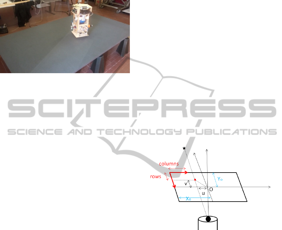
Given a point in the 3D space, its image is recorded
by a camera as a 2D point in the image plane. In a
digital image, the point on the image corresponds to
an element of an array, as in Figure 2. The
coordinates of the image center in the recorded array
of pixels, Xo and Yo in Figure 2, must be determined
by calibration (as it will be shown in Section 5).
Figure 2: Coordinates of a keypoint acquired by a camera.
The algorithm adopted to determine the position
and attitude is based on the hypothesis that an image
acquired at a given time is related by means of an
affine transformation to an image acquired at the
initial time (reference image). Let us call x and y the
coordinates of a keypoint (a “star”) in the reference
image, and u, v the coordinates of the same keypoint
in the current image. The relation between the
reference and the current keypoint including scale,
rotation and translation effects reads as:
cos sin
sin cos
x
y
t
xs s u
t
ys s v
θθ
θθ
⋅−⋅
=+
⋅⋅
(1)
where s is the scale factor,
θ
the rotation angle,
and
x
t ,
y
t
the translation between the current and the
VisualbasedNavigationofaFreeFloatingRobotbyMeansofaLabStarTracker
423
feature image. Considering all the N keypoints of the
reference image that have been associated to
keypoints of the current image, we can write:
1
11
1
11
10
cos
01
sin
...
... ... ... ...
10
01
x
N
NN
y
NN
N
x
uv
s
y
vu
s
t
x
uv
t
vu
y
θ
θ
−
⋅
⋅
=
−
(2)
Let us rewrite Eq. (2) as:
A=⋅uc
(3)
being
u the vector of keypoints of the current
image, A the matrix of reference keypoints,
c the
vector of the affine transform parameters. A least
square solution
c
can be found by performing the
pseudo-inverse (indicated by apex +) of the matrix
A,
A
+
=cu
(4)
Once the affine transformation parameters (i.e.,
θ
,
x
t ,
x
t , s) have been found, also the movement
performed by the camera (relevant to the times when
the reference and current images were acquired) can
be evaluated. In fact
θ
(i.e. the rotation between the
two images) clearly corresponds to the rotation of
the camera; the (planar) translation of the camera in
the 3D world is instead given by:
x
x
yy
Tfst
Tfst
=⋅⋅
=⋅⋅
(5)
where f is the ratio between the focal length of
the camera (in pixels) and the distance of the ceiling
from the camera (i.e. a conversion factor to be found
by calibration).
The main problems that characterize this
approach are basically two: first, it is necessary to
determine which point of an image is a keypoint (i.e.
a “star”). Next, it is necessary to associate the
corresponding keypoint in the reference image to
each keypoint in the current image.
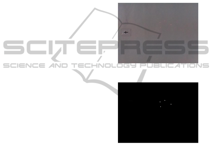
2.2 Identification of the Keypoints
At the scope of realizing a sufficient set of features,
red laser beams are pointed to the ceiling. It is
neither important the color of background surface
(white in this case), nor it is important that other
objects (a black cross in Figure 3) are in the camera
field of view. In fact, the laser footprints are so
bright that they result in a saturated point (close to a
perfect white) when acquired by the camera. The
image is therefore processed in order to determine
the mean value of the image array. A threshold is
selected so that only the pixels above the mean value
multiplied by the threshold are considered as
features. The threshold is dynamically adjusted at
the beginning of the maneuver in order to have a
proper acquisition of the reference image, in which
the known number of features must be present.
As a result, the processed image in Figure 4 is
obtained.
Figure 3: Image acquired by the LST, including the
keypoints and background clutter (black cross).
Figure 4: Keypoints resulting from the processing of the
acquired image.
2.3 Matching the Keypoints in
Tracking Mode
Space star trackers usually operate in two different
modes (Liebe, 2002). The first of them is the initial
attitude acquisition. Once an initial attitude has been
acquired, the star tracker switches to the tracking
mode. In this second mode, where the star tracker
has a priori knowledge, the database search can be
limited, allowing fast and accurate attitude
estimation. The LST developed for the planar
attitude and position determination is programmed
to work in a similar case.
ICINCO2015-12thInternationalConferenceonInformaticsinControl,AutomationandRobotics
424

First the initial image is acquired and stored as a
reference image. It is difficult however to match a
feature acquired in a different position and attitude
to the corresponding feature in the reference image.
In fact, the set of currently acquired keypoints
(vector
u in Eq. (3)) could be ordered in a different
way with respect to the reference keypoints (in
matrix A of Eq. (3)). Before performing the
evaluation of the affine transformation parameters in
Eq. (4), the current keypoint set must be reordered.
Differently from more advanced (but
computationally intensive) visual based methods,
such as SIFT or SURF (Lowe, 2004) the “star”
features are not characterized by identifiers, but
simply by their coordinates in the image plane.
Therefore it is not possible to discern between one
star and another one.
The approach proposed in this paper is therefore
to switch to a tracking mode where at each time step
k
t the current set of features is reordered by means
of a selection process based on the minimum
Euclidean distance between the keypoints belonging
to the current image and to the image acquired at the
previous time step
1k
t
−
. The hypothesis is in fact
that if the two images are taken at two very close
time steps (compared to the actual speed of the
camera), the corresponding features will be very
close in the two images – a hypothesis that is not
true if at a generic
k
t the keypoints are compared to
the reference image (acquired in
0
t ).
The reordered set of features is then saved to
serve as a benchmark at the following time
1k
t
+
. In
this way the keypoints order as extracted from the
reference image is propagated over time.
Once reordered, the current set of keypoints can
be compared with the reference set in order to solve
the problem in Eq. (4) for evaluating the affine
transformation parameters.
2.4 Dealing with False Stars
The approach described in the previous paragraph
manages to keep track of the movement of the stars
from the reference (initial) image to the currently
acquired image. However, a number of false features
could be present, corresponding to points in an
image that are misinterpreted as feature to be
tracked, or, inversely, “missing stars”, i.e. a
reference feature that for some reason is not present
in the current image. For example one of the laser
footprints could exit from the camera field of view,
or an incorrect tuning of the thresholds could lead to
identify as keypoints some bright points of the
background.
In these cases the number of currently acquired
keypoints is different from the number of reference
keypoints, and Eq. (4) cannot be solved. The
robustness of the algorithm has been increased by
implementing the following algorithm:
find the features (brightest points)
if (number of features now) equal to
or greater than (number of reference
features):
Discard the keypoints with larger
distance from the reference
keypoints
else:
Substitute the missing keypoint
with the corresponding one
recorded at the previous time
step.
The replacement of a keypoint with a previously
acquired keypoint decreases the accuracy of the
algorithm, but this detrimental effect is lesser as the
number of keypoints increases.
3 SIMULATION
The image processing, the algorithms for the
keypoint acquisition and reordering, the procedure
for false keypoints rejection, and finally the attitude
and position computation are firstly tested by means
of a software tool. A virtual set of features have been
modeled on a 640x480 array, taking the
characteristics of a really acquired image into
account. The “star” features are of different and time
varying shapes, as it is possible to see from Figure 5.
Moreover, for certain time intervals some of the
keypoints are artificially removed, and in some other
Figure 5: Numerical model for the simulation of the
acquired keypoints.
VisualbasedNavigationofaFreeFloatingRobotbyMeansofaLabStarTracker
425
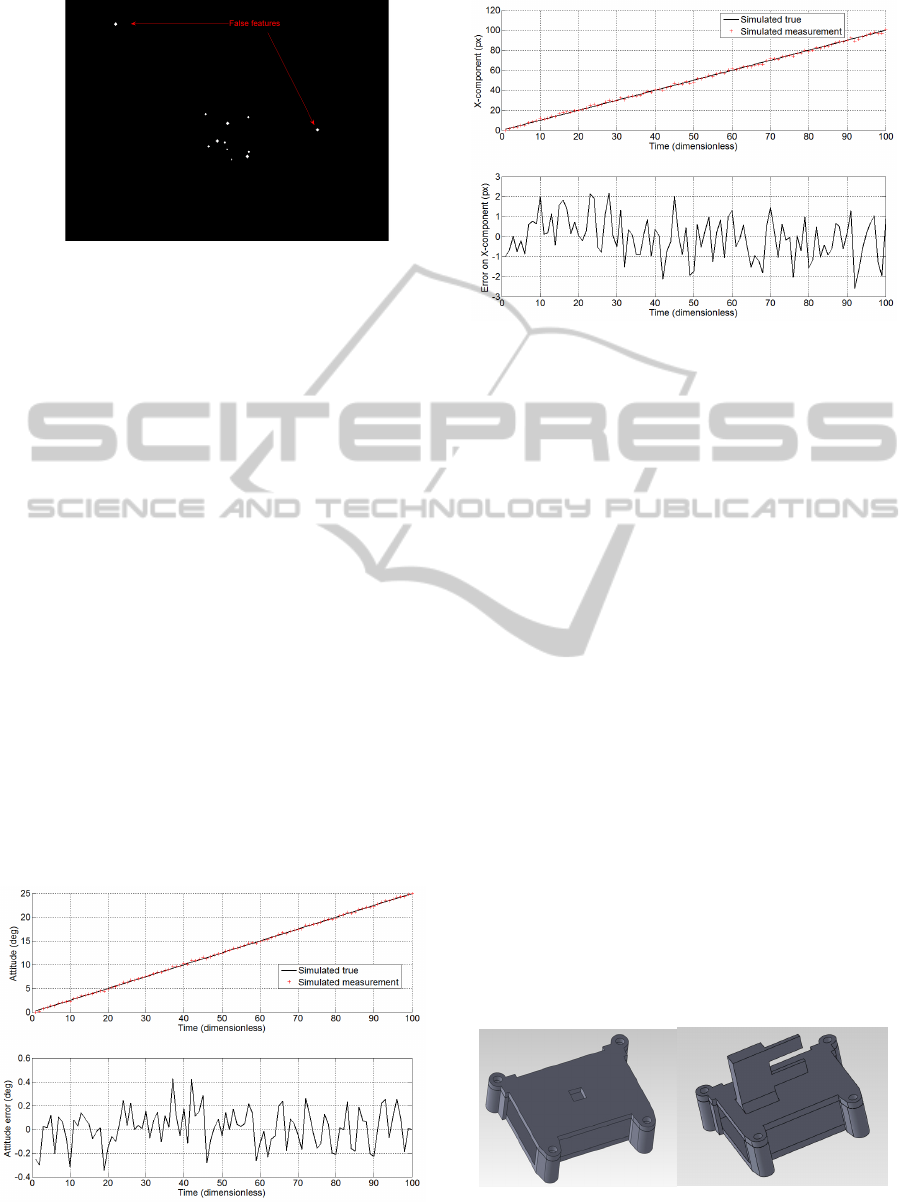
Figure 6: The software tool introduces varying brightness
of the keypoints, false keypoints and missing keypoints.
intervals false features are added, while applying a
translation and a rotation transformation to the
reference image (see Figure 6).
In details, a rotation of 0.25 deg per unit time
step (dimensionless in the simulation) has been
imposed, together with a translation in the X-
component. Figure 7 reports the simulated true
attitude behavior and the behavior of the rotation as
evaluated by means of Eq. (4) (upper subplot). The
error (lower subplot of Figure 7) is in the range of
0.5±
deg.
Regarding the computation of the translation,
Figure 8 reports the simulated true and the simulated
measured translation. The error in this case is
measured in pixels, and in the range of
approximatively
2± pixels.
The errors do not show any peak or sharp
variation when a feature is removed (from t = 15 to t
= 30) or when two false features are introduced
(from t = 45 to t = 60).
These results are quite promising and they could
be also improved by increasing the image resolution
or by using a larger number of features. For
example, passing from two features (bare minimum
Figure 7: Attitude behaviour (upper subplot) and attitude
error (lower subplot) in the simulated motion.
Figure 8: X-component behaviour (upper subplot) and X-
component error (lower subplot) in the simulated motion.
to solve Eq. (4), not allowing for any false feature
acquisition) to ten features means an improvement
of the attitude error from 0.41 deg (standard
deviation) to 0.12 deg, respectively.
4 DESIGN AND REALIZATION
OF THE LST
The LST has been designed to be an autonomous
device supplying position and attitude measurements
at the CPU query. At the scope, a Raspberry Pi
microprocessor has been selected for the image
acquisition and processing, since the required
algorithms are so simple that even with the limited
computational power of this board it is possible to
obtain a reasonable sampling time (5 Hz in the
experiments, with large margins for improvements).
A case has been realized with PLA plastic, following
the design in Figure 9. Different top elements have
been realized to accommodate a number of different
cameras; as an example, in Figure 10 the cases of a
PI Camera Module (upper subplot) and a Microsoft
LifeCam HD Cinema (lower subplot) are depicted.
The former camera offers a compact stowing, while
the second one has a better optics and autofocus
Figure 9: CAD design of the LST case for two possible
cameras, a Pi Camera Module (left) and a Microsoft
LifeCam (right).
ICINCO2015-12thInternationalConferenceonInformaticsinControl,AutomationandRobotics
426
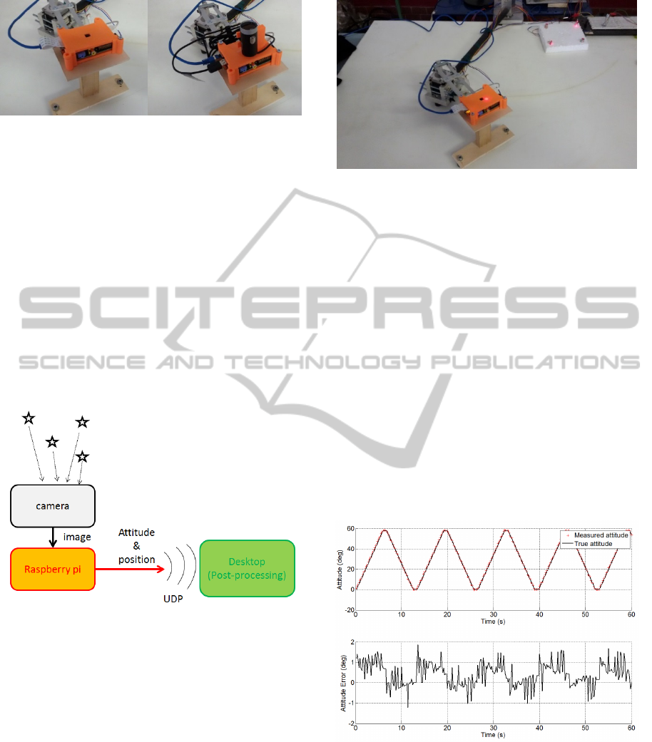
Figure 10: Actual realization of the LST with a Pi Camera
Module (left) and a Microsoft LifeCam (right).
capabilities. All the experiments have been
performed with the Pi Camera Module mounted.
The Raspberry Pi board has been programmed
via Matlab/Simulink. The C-code required to run on
the Linux release (Raspian) installed on the
microprocessor is automatically generated and
downloaded to the board. As shown in Figure 11, the
communication between the main processor (a
Desktop PC in this case, the free floating CPU in the
experiments involving the simulation of space-like
maneuvers) happens via UDP protocol; in the
current version a LAN cable is used, but in future
development a Wi-Fi communication will substitute
the physical link.
Figure 11: Data flow and software architecture for the
LST.
5 TESTS
For testing the LST, a two links planar manipulator
has been used, as shown in Figure 12. The
movements of its links are recorded by a shoulder
and an elbow encoder, with a resolution of 0.0003
deg and 0.0045 deg, respectively. This accuracy is
by far greater than the one expected from the
simulations reported in Section 4, and they will be
taken as the benchmark values for assessing the LST
performance. Four laser beams are used to create the
features on the lab ceiling.
Figure 12: The planar two-links manipulator used to move
the LST along predetermined paths.
5.1 Pure Rotation
As a first test, the LST is attached to the shoulder
joint. In this way, a pure rotation is assigned to the
system. A sequence of ramps from 0 deg to 60 deg
(and back) are assigned. The rotation is measured by
the shoulder encoder (benchmark value) and by the
LST. Figure 13 reports the two values (upper
subplot) and the difference between them (lower
subplot). The error is slightly higher than the one
expected from simulation. In fact the standard
deviation of the attitude error with four features is
0.23 deg in a simulation, while it is 0.6 in the
experiment. This difference was expected, since the
visual navigation suffers from a number of
disturbances (varying light conditions, background
clutter and so on) which can be hardly modeled in a
simulation environment.
Figure 13: Attitude behaviour (upper subplot) and attitude
error (lower subplot) for the experiment involving pure
rotation.
This experiment has been also used for a
calibration of the camera. In fact, as explained in
Section 2, in a camera the image center does not
coincide with the center of the array; referring back
to Figure 2, this means that in a 640x480 image, the
VisualbasedNavigationofaFreeFloatingRobotbyMeansofaLabStarTracker
427
coordinates of the point O are not necessarily
320x240. This fact has an important effect when the
measurements of the translation must be evaluated.
When a pure rotation is imposed to the LST, the
evaluation of the affine transformation parameters
for a non-calibrated camera will result in a rotation
(correctly computed) plus a residual translation. A
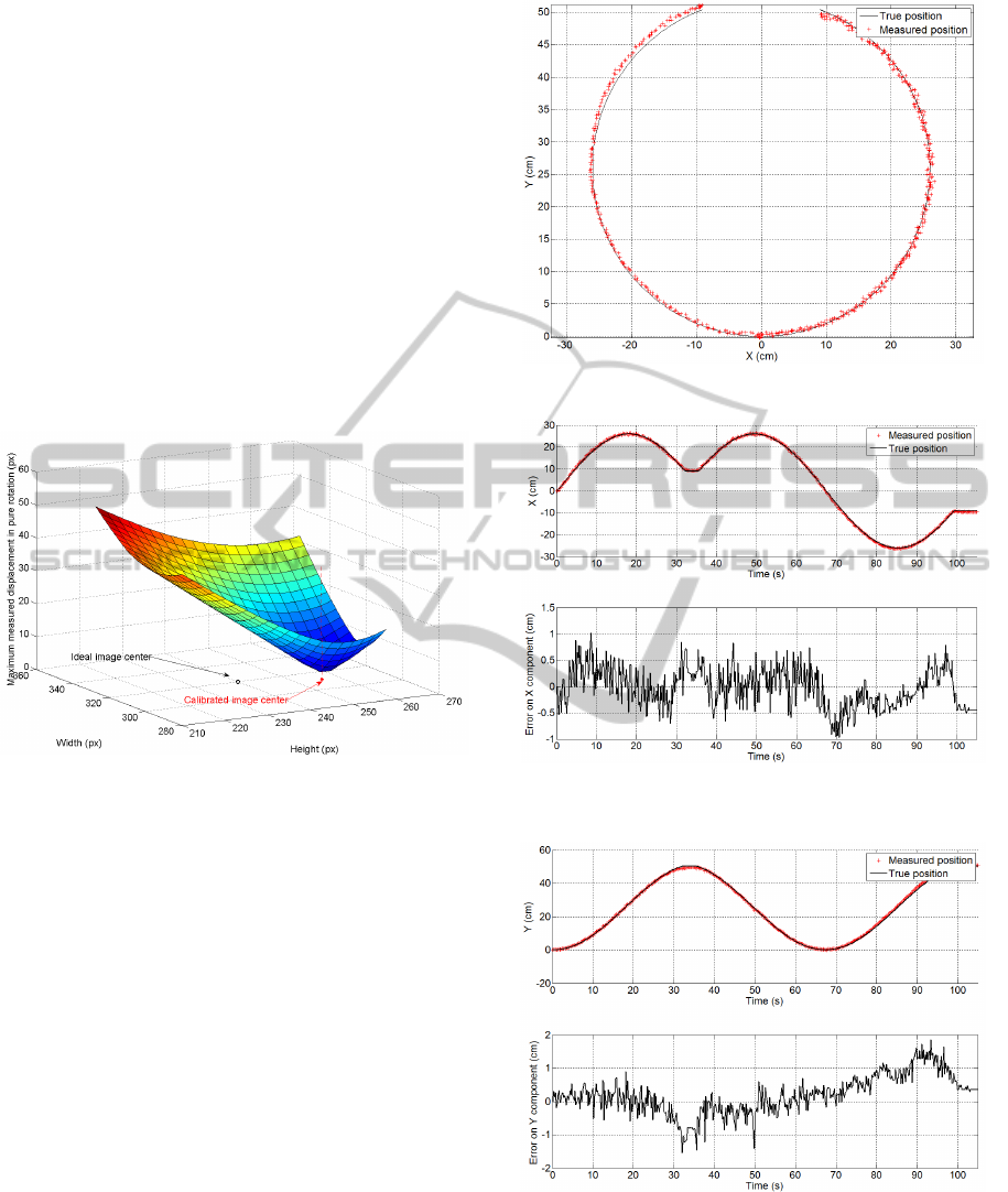
simple calibration has been therefore performed (a
more complete one could be found in (Zhang, 2002))
by acquiring the keypoints once, and then post-
processing them with a number of different values of
the possible image center coordinates. For each
tentative center the maximum value of the norm of
the residual translation is recorded. The coordinates
of the center that allow for a minimum – ideally zero
– norm of the translation (see Figure 14) is the real
image center.
Figure 14: Result of the procedure to determine the image
centre by means of a calibration procedure.
5.2 Translation and Rotation
The final experiment consists in a coupled rotation
and translation of the LST device. At the scope, it is
placed at the end of the second link, which is moved
along a circular trajectory by moving the elbow
motor between +160 deg and -160 deg. The true and
measured trajectories are reported in Figure 15,
where the selected reference frame is coincident
with a reference frame attached to the camera at the
initial time.
The attitude behaviour is not reported, since the
accuracy is of the same order as in the pure rotation
experiment. The X and Y translation (in the real
world) are plotted in Figure 16 and Figure 17,
respectively. From the upper subplot of the two
figures it is possible to compare the true and
measured components of the translation. The lower
subplots report the errors. The standard deviation is
0.4 cm for X component and 0.57 cm for the Y
component, while the maximum errors (absolute
Figure 15: True and measured trajectory.
Figure 16: X-component behaviour (upper subplot) and X-
component error (lower subplot) in the experiment.
Figure 17: Y-component behaviour (upper subplot) and Y-
component error (lower subplot) in the experiment.
value) are 1.0 cm for the X component and 1.8 cm
for the Y component. Even though the device is
currently under development, these values are quite
promising and could allow an accurate and safe
ICINCO2015-12thInternationalConferenceonInformaticsinControl,AutomationandRobotics
428

navigation for a large number of space experiments,
taking into account the possibility to implement data
fusion algorithms including the inertial
measurements.
6 CONCLUSIONS
A device has been developed for the navigation of a
free floating platform, dedicated to experiments
involving space operations. The device has been
named Lab Star Tracker (LST) since, like a space
star tracker, it uses a set of features acquired by
means of a camera in order to determine its attitude.
Differently from the space star trackers, also the
position with respect to an inertial frame can be
determined. The working principles at the basis of
the LST have been reported, together with the
algorithms that are required to make the system
robust with respect to false acquisitions and missed
acquisitions. The performance of the system has
been first simulated by means of a dedicated
software tool which reproduces the image of the
features, and then tested by means of an
experimental setup. A planar two-links manipulator
has been used to move the LST along known
trajectories. The LST measurements have been
compared with the true trajectory, and the
performance in terms of attitude and position
accuracy have been established. In details, an error
below 1deg and 1cm have been found for attitude
and position, which is a level of accuracy that can be
satisfactory for a large number of operational
scenarios. Future developments of the LST will
consist in adding a Wi-Fi link, and increasing the
image resolution up to high definition levels,
maintaining an acceptable sample time. Finally, the
influence of the keypoints distribution should be
studied, in order to find optimal “constellations” that
allow for a minimization of the navigation error.
REFERENCES
Gasbarri, P., Sabatini, M., Leonangeli, N., Palmerini,
G.B., 2014. Flexibility issues in discrete on–off
actuated spacecraft: Numerical and experimental tests,
Acta Astronautica, Volume 101, August–September
2014, Pages 81-97.
Sabatini, M., Palmerini, G. B., Gasbarri, P., 2014. A
testbed for visual based navigation and control during
space rendezvous operations, International
Astronautical Congress, Toronto, Canada, October
2014.
Xu, W., Liang, B., Xu, Y., 2011. Survey of modeling,
planning, and ground verification of space robotic
systems, Acta Astronautica, Vol.68, No.11–12, pp.
1629-1649.
Menon, C. Aboudan, A., Cocuzza, S., Bulgarelli, A.,
Angrilli, F., 2005. Free-flying robot tested on
parabolic flights: kinematic control, Journal of
Guidance, Control, and Dynamics, Vol.28, No.4,
pp.623–630.
Fujii, H.A., Uchiyama, K., 1996. Ground-based simulation
of space manipulators using test bed with suspension
system, Journal of Guidance, Control, and Dynamics,
vol. 19, No. 5, pp. 985–99.
Benninghoff, H., Tzschichholz, T., Boge, T., Rupp, T.,
2011. Hardware-in-the-Loop Simulation of
Rendezvous and Docking Maneuvers in On-Orbit
Servicing Missions, 28th International Symposium on
Space Technology and Science, Okinawa.
Schwartz, J. L., Peck, M. A., Hall, C. D., 2003. Historical
Review of Air-Bearing Spacecraft Simulators, Journal
of Guidance, Control and Dynamics, Vol. 26, No. 4.
Sidi, M. J., 1997. Spacecraft Dynamics and Control: A
Practical Engineering Approach, Cambridge
University Press, ISBN: 0-512-55072-6.
Shuster, M. D. and Oh, S. D., 1981. Three-Axis Attitude
Determination from Vector Observations, Journal of
Guidance and Control, Vol. 4, No. 1, pp. 70-77.
Delabie, T., De Schutter, J., and Vandenbussche, B., 2013.
A Highly Efficient Attitude Estimation Algorithm for
Star Trackers Based on Optimal Image Matching,
Journal of Guidance, Control, and Dynamics, Vol. 36,
No. 6, pp. 1672-1680.
Liebe, C. C., 2002. Accuracy Performance of Star
Trackers - A Tutorial, IEEE Transactions on aerospace
and electronic systems, Vol. 38, No. 2.
Lowe, D.G.. Distinctive Image Features From Scale-
invariant keyp.
Zhang, Z., 2002. A Flexible New Technique for Camera
Calibration, IEEE Transactions on Pattern Analysis
And Machine Intelligence, Vol. 22, No. 11.
VisualbasedNavigationofaFreeFloatingRobotbyMeansofaLabStarTracker
429
