Control of Three-Phase Grid-Connected Microgrids using Artificial
Neural Networks
Shuhui Li
1
, Xingang Fu
1
, Ishan Jaithwa
1
, Eduardo Alonso
2
, Michael Fairbank
2
and Donald C. Wunsch
3
1
Department of Electrical and Computer Engineering, the University of Alabama, Tuscaloosa, AL, U.S.A.
2
Department of Computer Science, City University London, London, U.K.
3
Department of Electrical and Computer Engineering, Missouri University of Science and Technology, Rolla, MO, U.S.A.
Keywords: Neural Network Control, Microgrid, Distributed Energy Resources, Grid-Connected Converter.
Abstract: A microgrid consists of a variety of inverter-interfaced distributed energy resources (DERs). A key issue is
how to control DERs within the microgrid and how to connect them to or disconnect them from the microgrid
quickly. This paper presents a strategy for controlling inverter-interfaced DERs within a microgrid using an
artificial neural network, which implements a dynamic programming algorithm and is trained with a new
Levenberg-Marquardt backpropagation algorithm. Compared to conventional control methods, our neural
network controller exhibits fast response time, low overshoot, and, in general, the best performance. In
particular, the neural network controller can quickly connect or disconnect inverter-interfaced DERs without
the need for a synchronization controller, efficiently track fast-changing reference commands, tolerate system
disturbances, and satisfy control requirements at grid-connected mode, islanding mode, and their transition.
1 INTRODUCTION
Distributed generation (DG) is an approach that
employs small-scale technologies to produce
electricity close to the end users of power. DG
technologies often consist of modular and
renewable-energy generators. They offer a number
of potential benefits over traditional power
generators, such as lower-cost electricity and
increased power reliability and security with fewer
environmental consequences. A microgrid is defined
as an interconnected network of distributed energy
systems (loads and DG resources) that can function
with or without a connection to the main grid. This
new approach to designing and building future smart
grids focuses on creating a plan for local energy
delivery that meets the needs of the constituents
being served. Microgrids can efficiently integrate
small-scale DGs into low-voltage (LV) systems and
supply the demand of local customers, so their
development is expected to yield the following
benefits: 1) enable the development of sustainable
and green electricity; 2) enable larger public
participation in the investment in small-scale
generation; 3) reduce the number of marginal central
power plants, 4) improve the security of the supply;
5) reduce losses; and 6) enable better network
congestion management and control to improve
power quality. One important issue in microgrid
operation is how to control the inverter-interfaced
distributed energy resources (DERs). Conventionally,
these DERs are controlled using standard vector
control technology (mostly, Proportional Integral, PI,
controllers). Within this framework, different
solutions for connecting them to and disconnecting
them from the main network have been proposed
(Blaabjerg et al., 2006). Specifically, implementing
a fast and accurate grid voltage synchronization
algorithm (Rodríguez et al., 2012) is crucial, though
this usually involves a complicated process. Recent
studies have shown that an artificial neural network
can be trained and used to control a grid-connected
converter (Li et al., 2014). In (Li et al., 2014), the
neural network performance was evaluated mainly
for d- and q-axis current tracking control of a
grid-connected converter in a vector control
condition. Compared to conventional vector control
methods, the neural network yielded an extremely
fast response time, low overshoot, and, in general,
the best performance. The purpose of this paper is to
investigate neural network control technology for
control of grid-connect converters, including PQ and
PV converters, and for control of a microgrid
58
Li, S., Fu, X., Jaithwa, I., Alonso, E., Fairbank, M. and Wunsch, D..
Control of Three-Phase Grid-Connected Microgrids using Artificial Neural Networks.
In Proceedings of the 7th International Joint Conference on Computational Intelligence (IJCCI 2015) - Volume 3: NCTA, pages 58-69
ISBN: 978-989-758-157-1
Copyright
c
2015 by SCITEPRESS – Science and Technology Publications, Lda. All rights reserved

containing PQ and PV grid-connected converters.
The main contributions of the paper include: 1) a
neural network vector control strategy for optimal
control of grid-connected converters (GCC); 2) a
neural network design and training algorithm that
can handle GCC control properly under physical
system constraints; 3) control of inverter-interfaced
DERs in a microgrid without using a
synchronization control technique; and 4)
investigation of neural network vector control for a
microgrid network.
2 CONTROL ARCHITECTURES
The control objective of a DER is to manage the
active power transferred from the dc side to the ac
side and to control the reactive power absorbed from
the ac grid. This active and reactive power control
usually is transformed into d- and q-axis current
control (Li et al., 2011). In the d-q reference frame
and using the motor sign convention, the voltage
balance across the grid filter is:
v
d
v
q
⎡
⎣
⎢
⎢
⎤
⎦
⎥
⎥
= R
f
i
d
i
q
⎡
⎣
⎢
⎢
⎤
⎦
⎥
⎥
+ L
f
d
dt
i
d
i
q
⎡
⎣
⎢
⎢
⎤
⎦
⎥
⎥
+
ω
s
L
f
−i
q
i
d
⎡
⎣
⎢
⎢
⎤
⎦
⎥
⎥
+
v
d1
v
q1
⎡
⎣
⎢
⎢
⎤
⎦
⎥
⎥
(1)
in which v
d
and v
q
represent the Point of
Common Coupling (PCC) d- and q-axis voltages, i
d
and i
q
are the d- and q-axis currents from the grid to
the DER,
ω
s
is the angular frequency of the PCC
voltage, and v
d1
and v
q1
are the inverter’s d- and
q-axis output voltages. L
f
and R
f
are the inductance
and resistance of the grid filter, respectively. Using
the PCC voltage-oriented frame (Li et al., 2011; Li
et al., 2014), the instant active and reactive powers
absorbed by the DER from the grid are proportional
to the grid's d- and q-axis currents, respectively, as
shown by Eqs. (2) and (3):
p(t) = v
d
i
d
+ v
q
i
q
= v
d
i
d
q(t) = v
q
i
d
− v
d
i
q
=−v
d
i
q
(2)
(3)
2.1 Conventional Control Structure
The conventional standard vector control method of
a DER converter implements a nested-loop structure.
The control strategy of the inner current loop is
developed by rewriting Eq. (1) as:
(
)
1dfdfd sfqd
vRiLdidt Liv
ω
=+⋅ − +
(4)
(
)
1qfqfq sfd
v R i L di dt L i
ω
=+⋅ +
(5)
in which the expressions in parentheses are
treated as the state equations between the voltage
and current on the d- and q-axis loops, and the
remaining expressions are treated as compensation
terms (Li et al., 2011; Rocabert et al., 2011). The
final control voltages,v
d1
*
and v
q1
*
, applied to the
DER converter include the d- and q-axis voltages, v
d
’
and v
q
’
, generated by the current-loop controllers, in
addition to the compensation terms, as shown in Eq.
(6). Hence, the conventional control configuration of
the DER converter intends to regulate i
d
and i
q
using
v
d
’
and v
q
’
, respectively. However, as indicated in (Li
et al., 2011), v
d
’
is only effective for reactive power,
or i
q
, control, and v
q
’
is only effective for active
power, or i
d
, control. Although the final control
voltage applied to the converter contains the
compensation terms, those compensation terms are
not generated by the PI controllers.
*' *'
11
,
ddsfqdqqsfd
vv Livvv Li
ωω
=− + =+
(6)
2.2 Neural Network Control Structure
Following (Li et al., 2011), our neural network
vector control structure of a DER a d-axis loop is
used for active power control and a q-axis loop is
used for reactive power, or grid voltage support
control. The error signal between the measured and
reference active power generates a d-axis current
reference to the neural network through a PI
controller, while the error signal between the actual
and desired reactive power generates a q-axis current
reference. The neural network, known here as the
action network, is applied to the DER inverter
through a pulse width modulation (PWM)
mechanism to regulate the DER output voltage in
the three-phase ac system. The ratio of the inverter
output voltage to the output of the action network is
a gain of k
PWM
, which equals V
dc
/2 if the amplitude
of the triangle voltage waveform in the PWM
scheme is 1V (Mohan et al., 2002). The integrated
DER system, described by Eq. (1), is rearranged into
the standard state-space representation using Eq. (7),
in which the system states are i
d
and i
q
, PCC voltages
v
d
and v
q
normally are constant, and converter output
voltages v
d1
and v
q1
are the control voltages to be
specified by the output of the action network. For
digital control implementation and offline training of
the neural network, the discrete equivalent of the
continuous system state-space model, Eq. (7), must
be obtained using Eq. (8), in which T
s
represents the
Control of Three-Phase Grid-Connected Microgrids using Artificial Neural Networks
59
sampling period, k is an integer time step, F is the
system matrix, and G is the matrix associated with
the control voltage. In this paper, a zero-order-hold
discrete equivalent (Franklin et al., 1998) is used to
convert the continuous state-space model of the
system in Eq. (7) to the discrete state-space model in
Eq. (8). In all experiments, T
s
=1ms.
d
dt
i
d
i
q
⎡
⎣
⎢
⎢
⎤
⎦
⎥
⎥
=−
R
f
L
f
−
ω
s
ω
s
R
f
L
f
⎡
⎣
⎢
⎢
⎤
⎦
⎥
⎥
i
d
i
q
⎡
⎣
⎢
⎢
⎤
⎦
⎥
⎥
−
1
L
f
v
d1
v
q1
⎡
⎣
⎢
⎢
⎤
⎦
⎥
⎥
+
1
L
f
v
d
v
q
⎡
⎣
⎢
⎢
⎤
⎦
⎥
⎥
(7)
i
d
kT
s
+ T
s
()
i
q
kT
s
+ T
s
()
⎡
⎣
⎢
⎢
⎢
⎤
⎦
⎥
⎥
⎥
= F
i
d
kT
s
()
i
q
kT
s
()
⎡
⎣
⎢
⎢
⎢
⎤
⎦
⎥
⎥
⎥
+ G
v
d1
kT
s
()
− v
d
v
q1
kT
s
()
− v
q
⎡
⎣
⎢
⎢
⎢
⎤
⎦
⎥
⎥
⎥
(8)
The action network is a fully connected
multi-layer perceptron (Hagan et al., 2002) with six
input nodes, two hidden layers having six nodes
each, two output nodes, and shortcut connections
between all pairs of layers, with hyperbolic tangent
functions at all nodes. These six input components
correspond to 1) the d- and q-axis current signals, 2)
the two error signals of the d- and q-axis currents,
and 3) the two integrals of the error signals. To
simplify the expressions, the discrete system model
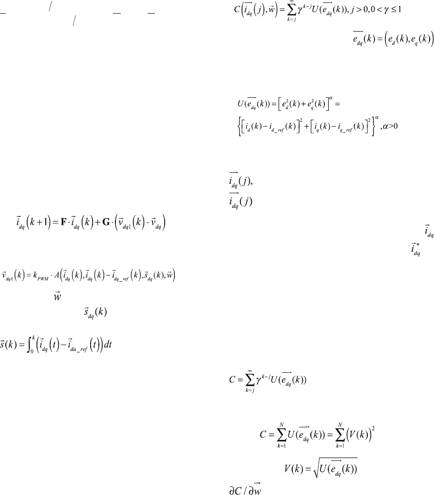
in Eq. (8) is represented by:
(9)
For a reference dq current, the control action
applied to the system is expressed by:
(10)
in which
represents the weight vector of the
action network, and
represents the network’s
integral input vector defined by
. To prevent the neural
network controller from being affected by the PCC
voltage variation, we used a strategy that introduces
the disturbance PCC voltage to the output of the
network.
3 NEURAL NETWORK
TRAINING
Unlike the conventional standard vector controller,
the neural network controller is produced through
training using Dynamic Programming (DP). DP
employs Bellman’s Principle of Optimality (Bellman,
1957) and is a very useful tool for solving optimal
control problems (Balakrishnan and Viega, 1996; He
et al., 2012). The typical structure of discrete-time
DP includes a discrete-time system model and a
performance index or cost associated with the
system (Wang et al., 2009). The DP cost function
associated with the vector-controlled system is
defined as:
(11)
whith
γ
a discount factor,
= i
d
(k) − i
d _ ref
(k), i
q
(k) − i
q_ ref
(k)
(
)
and
U
is
defined as:
(12)
in which
α
is a constant. The function
C(
⋅
),
depending on the initial time
j
and the initial state
is referred to as the cost-to-go of state
of the DP problem. The objective of the
neural network controller is to solve a current
tracking problem, i.e., to hold the existing state
near a given (possibly moving) target state
so
that the function
C
(
⋅
)
in Eq. (11) is minimized. The
current-loop action network was trained to minimize
the DP cost in Eq. (11) using Levenberg-Marquardt
backpropagation (LMBP) (Hagan et al., 2002).
LMBP, a variation of Newton’s method, minimizes
a function that is the sum of squares of a nonlinear
function. Using LMBP with a general value for
α
requires a modification for the cost function
()C
⋅
defined in Eq. (11). Consider the cost function
, in which
γ
= 1,
1,=j
and
k
=
1,,
N
.
Then,
C can be written as:
(13)
in which
and the gradient
can be written in matrix form as:
NCTA 2015 - 7th International Conference on Neural Computation Theory and Applications
60
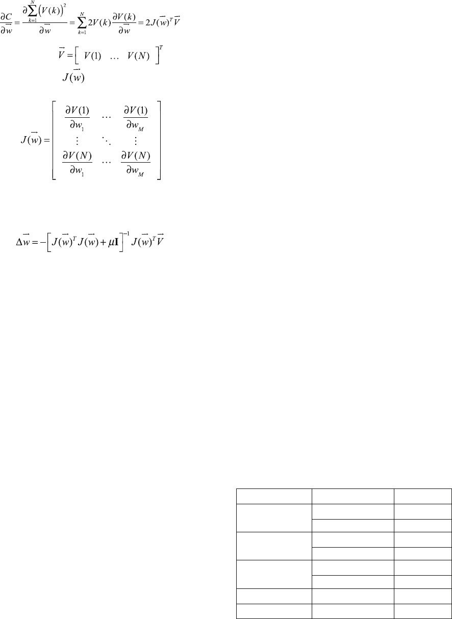
(14)
in which
, and the
Jacobian matrix
is:
(15)
Therefore, the process of updating the weights
using LMBP for a neural network controller can be
expressed as:
(16)
The parameter
μ
was dynamically adjusted to
ensure that the training followed the decreasing
direction of the cost function. When
μ
increased,
(16) approached the steepest descent algorithm with
a small learning rate, while as
μ
decreased, the
algorithm (16) approached Gauss-Newton, which
typically provides faster convergence. In order to
increase the speed of computation, the weight update
in Eq. (16) was conducted using Cholesky
factorization, which is roughly twice as efficient as
lower-upper decomposition for solving systems of
linear equations (Press et al., 1992).
To train the action network, the system data
associated with Eq. (7) had to be specified. The
training procedure for the current-loop action
network involved: 1) randomly generating a sample
initial state i
dq
(j); 2) randomly generating a changing
sample reference dq current time sequence; 3)
unrolling the trajectory of the system from the initial
state; 4) training the current-loop neural network
based on Eq. (16); and 5) repeating the process for
all of the sample initial states and reference dq
currents until reaching a stop criterion associated
with the DP cost. All of the network weights initially
were randomized using a uniform distribution with
zero mean and 0.1 variance.The generation of the
reference current considered the physical constraints
of a practical DER inverter system. The randomly
generated d- and q-axis reference currents first were
chosen uniformly from [-I
rated
,I
rated
], in which I
rated
represents the rated inverter line current. Then, these
randomly generated d- and q-axis current values
were checked and modified to ensure that their
resultant magnitude did not exceed the inverter’s
rated current limit and/or the control voltage did not
exceed the converter’s PWM saturation limit. From
the neural network standpoint, the PWM saturation
constraint indicates the maximum positive or
negative voltage that the action network can output.
Therefore, if a reference dq current requires a
control voltage that exceeds the acceptable voltage
range of the action network, it is impossible to
reduce the cost during the training of the action
network. The neural network controller is trained
offline, and no training occurs in the real-time
control stage. Without online training, a real-time
control action can be computed very quickly using
modern DSP chips. The most important issue is the
sampling time. However, an optimal neural network
controller can be trained using a large sampling time
based on the DP principle, while tuning a
conventional controller for the same sampling time
could be very difficult or impossible. Therefore, the
neural network controller actually has lesser
sampling and computing power requirements during
the real-time control process.
4 CONTROL OF INVERTER DER
The key requirements for controlling
inverter-interfaced DERs within a microgrid include:
1) active power control; 2) reactive power control;
3) grid voltage support control, and 4) control under
physical constraints. If a GCC can meet these
control requirements, it can be applied broadly to
power and energy system applications involving
GCCs. In our experiments, the system data and
controller parameters for various control purposes
are as in Tables 1 and 2:
Table 1: Systems data.
Component Parameter Value
AC system
Line voltage
400V
Frequency
60Hz
Transmission line
Resistance
0.0076Ω
Inductance
0.154mH
Grid-filter
Resistance
0.006Ω
Inductance
1mH
DER converter Switching frequency
3000Hz
DC system Voltage
700V
Control of Three-Phase Grid-Connected Microgrids using Artificial Neural Networks
61

Table 2: Parameters of DER controller (k
p
– proportional
gain, k
i
– integral gain).
Approach Controller
Gain (k
p
/ k
i
)
Conventional
Current loop
1.54 / 53.52
AC bus voltage 1.09 / 35.6
Neural network
Current loop Neural network
AC bus voltage 1.09 / 35.6
The PCC bus was connected to the microgrid
through a transmission line that was modeled by an
impedance. A fault-load was connected before the
PCC bus to evaluate how the controller behaves
when a fault appears in the grid. The DER inverter’s
switching frequency was 3kHz. Typical strategies
for operating a DER in a microgrid include
PQ-inverter DER and PV-inverter DER (Katiraei et
al., 2008). In the power converter switching
condition, the controller can be evaluated under
close to real-life conditions. The position of the PCC
voltage space vector
θ
v
was obtained directly from
the PCC voltage measurement in the α-β reference
frame given by:
θ
v
= tan
−1
v
α
v
β
()
(17)
4.1 Control of PQ-Inverter DERs
A PQ-inverter DER operates by injecting active and
reactive power into the microgrid. The active and
reactive power control at the PCC of an
inverter-interfaced DER is converted to d- and
q-axis current control. The d- and q-axis current
references, i
d
*
and i
q
*
, are obtained either through a
PI control mechanism or by calculating Eqs. (2) and
(3), as discussed in (Li et al., 2011):
** * *
,
d acd q acd
iPv i Qv==−
(18)
The desired active power of the DER normally is
generated according to either a maximum power
capture rule for a renewable DER unit or an active
power control demand from the microgrid central
control (MGCC) level. The desired reactive power is
issued either locally for the unity power factor or
centrally according to a control command from the
MGCC.
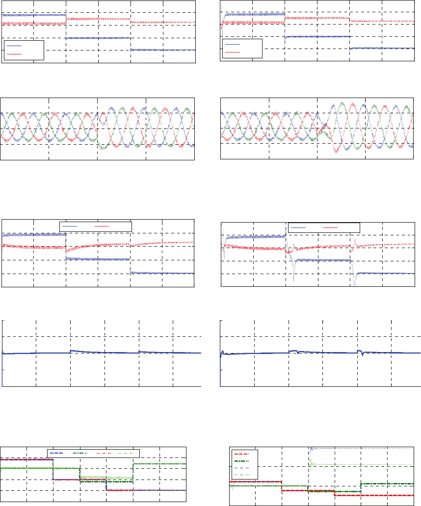
Fig. 1 in the Appendix presents a case study of
the PQ-controlled DER using the conventional and
neural network control methods. At first, the active
and reactive power references were 40kW and
0kVar, respectively. After the system started, the
neural network controller quickly regulated the
active and reactive power of the DER to the
reference values. When the reference power took on
new values of -50kW/20kVar and -100kW/10kVar
at t=2sec and t=4sec, respectively, the neural
network controller immediately restored DER power
to the new reference values (Fig. 1a). As shown in
Fig. 1c, the three-phase grid current was properly
balanced. For any other commanded change of the
reference power within the DER-rated power limit,
the system could be adjusted immediately to the new
reference power, demonstrating the strong optimal
control capability of the neural network vector
controller. Compared to the neural network
controller, the conventional controller was slower,
had a higher oscillation, and took longer to reach its
target value. This was more evident at t=0sec when
starting the system.
4.2 Control of PV-Inverter DERs
One critical disadvantage of the PQ-inverter DER is
that the PCC bus voltage changes as active and
reactive power are transferred through the PCC and
as the load varies. A PV-inverter DER operates by
injecting active power into the microgrid while
simultaneously maintaining the PCC bus voltage at a
desired value. The desired active power is formed in
the same way as that used in a PQ-inverter DER, but
the reactive power is controlled according to the
error signal between the desired and the actual PCC
bus voltage to which the inverter is connected.
Therefore, as the PCC bus voltage fluctuates, so
does the reference q-axis current generated by a PI
controller.
Fig. 2 in Appendix presents a case study of the
PV-inverter DER using the conventional and neural
network controllers. The active power reference was
the same as that used in the case study presented in
Fig. 1, while the reference PCC voltage was 1pu.
After the system started, the neural network
controller quickly regulated the active power of the
DER and the PCC bus voltage to the reference
values. The inverter initially absorbed active power
from the grid, and the reactive power was generated
so as to maintain the PCC voltage at 1pu. When the
reference active power in the ac system began to
generate at t=2sec, the reactive power shifted from
generating to absorbing. At t=4sec, the reactive
power absorbed more in order to maintain the PCC
voltage for the increased active power generated by
the DER (Fig. 2a). Similar to Fig. 1, this case study
demonstrates the excellent performance of the neural
network vector controller for the PV-inverter DER.
However, using the conventional controller, a large
oscillation occurred each time the DER active power
NCTA 2015 - 7th International Conference on Neural Computation Theory and Applications
62
changed significantly (Fig. 2b).
4.3 Control of DER Inverter under
Constraints
In practice, a DER inverter cannot operate beyond
the rated power and PWM saturation of the
converter. To handle DER operation under such
conditions, we propose controlling the DER by
maintaining the effectiveness of the active power
control while meeting the reactive power control
demand as much as possible. This is expressed as:
minimize
Q
ac
− Q
ac
*
, subject to
P
ac
= P
ac
*
i
d
2
+ i
q
2
≤ I
rated
,
v
d1
2
+ v
q1
2
3
≤
V
dc
22
⎧
⎨
⎪
⎪
⎩
⎪
⎪
.
For the conventional controller, the following
strategies are used. To prevent the DER converter
from exceeding the PWM saturation limit, Eq. (19)
is applied if the amplitude of the reference voltage
generated by the inner current-loop controller
exceeds the converter’s PWM saturation limit
(Gagnon, 2009; Li et al., 2011), in which v
d1_new
*
and
v
q1_new
*
are the d and q components of the modified
controller output voltage, and V
max
is the maximum
allowable dq voltage:
v
d1_ new
*
= V
max
cos ∠v
dq1
*
()
v
q1_new
*
= V
max
sin ∠v
dq1
*
()
(19)
To prevent the DER converter from exceeding
the rated current, Eq. (20) is employed if the
amplitude of the reference current generated by the
outer control loop exceeds the rated current limit, i.e.,
the d-axis current reference i
d
*
is kept constant to
maintain active power control effectiveness, while
the q-axis current reference i
q
*
is modified to satisfy
the reactive power or ac system bus voltage support
control demand as much as possible (Gagnon, 2009;
Li et al., 2011):
i
d _ new
*
= i
d
*
i
q_ new
*
= sign i
q
*
()
⋅ i
dq _max
*
()
2
− i
d
*
()
2
(20)
For the neural network controller, if |i
dq
*
|
generated by the dc-voltage or the active and
reactive power control loops exceeds the rated
current limit, i
d
*
and i
q
*
are modified by Eq. (20)
before being applied to the action network (Li et al.,
2011); if |v
dq1
*
| generated by the current control
loops exceeds the PWM saturation limit, the action
neural network automatically turns into a state by
regulating v
q1
to maintain the effectiveness of the
active power control while restraining v
d1
to meet the
reactive power control demand as much as possible.
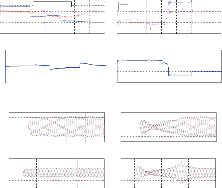
Fig. 3 in the Appendix presents a case study of
the PQ-inverter DER in which there was high
demand for reactive power generation. The active
power reference was the same as that used in the
case study illustrated in Fig. 2, while the reactive
power demand caused the required control voltage to
exceed the inverter’s PWM saturation limit at
t=3sec. As Fig. 3a illustrates, the neural network
controller automatically restrained the reactive
power control while maintaining the effectiveness of
the active power control at t=3sec. At t=5sec, when
the reactive power demand generation decreased,
causing the control voltage to fall below the PWM
saturation limit, the neural network controller
returned to its normal control condition immediately.
For the conventional controller, however, when the
control voltage exceeded the inverter’s PWM
saturation limit at t=3sec, the system could not
follow the control commands properly due to its
competing control nature (Li et al., 2011), as shown
in Fig. 3b.
Fig. 4 in the Appendix presents a case study of
the PV-inverter DER for PCC voltage support
control under a moderate voltage drop caused by a
fault at t=3sec. Due to the inverter’s PWM saturation
constraint, the neural network controller could not
maintain the PCC voltage at 1pu to compensate for
the voltage drop (Fig. 4c). Instead, it operated by
maintaining the effectiveness of the active power
control while providing PCC voltage support control
as much as possible. At t=5sec, when the short
circuit was cleared, the neural network controller
returned to its normal operating condition, and the
PCC bus voltage recovered to the rated bus voltage
quickly, thus demonstrating the neural network
controller’s excellent PCC voltage support control
under the physical constraints of DERs. For the
conventional controller, however, when the required
control voltage exceeded the inverter’s PWM
saturation limit shortly after t=3sec, the system
could not follow the control commands properly, as
shown in Fig. 4b and 4d.
5 MICROGRID CONTROL AND
STABILITY ANALYSIS
5.1 A Benchmark Microgrid Network
A typical benchmark low-voltage (LV) microgrid
Control of Three-Phase Grid-Connected Microgrids using Artificial Neural Networks
63
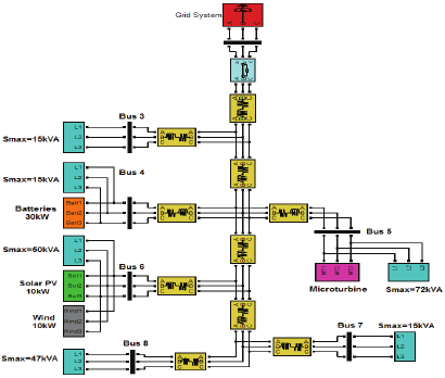
network was built using MatLab SimPowerSystems
and an Opal-RT real-time simulation system, as
shown in Fig. 5. The microgrid was supplied
through a LV feeder to serve a suburban residential
area with a limited number of consumers connected
along its length. The microgrid consisted of DGs
from the most relevant technologies, such as solar
photovoltaics, wind turbines, microturbines, and fuel
cells. The impedance data for various line types used
in the network, as well as detailed information about
the installed capacities of the microturbine, fuel cell,
and battery storage device, are available in
(Papathanassiou et al., 2005)). The loads were
assumed to have similar load patterns. The power
factor was 0.85 lagging. The DGs were connected to
the following buses: solar on buses 6 and 7, wind on
bus 6, microturbine on bus 5, fuel cell on bus 8, and
battery on bus 4. Thus, the benchmark network
maintained the important technical characteristics of
real-life utility distribution systems, while
dispensing with the complexity of actual networks,
to permit the efficient modeling and simulation of
the microgrid’s operation.
Figure 5: Benchmark LV microgrid networks using neural
controllers.
5.2 DER Synchronization
Before connecting any DER to the microgrid, it must
be synchronized accurately with the network voltage
to avoid over currents (Rodríguez et al., 2012). Most
grid-tied systems use a phase locked loop (PLL) for
synchronization (Rodríguez et al., 2012). Many grid
synchronization applications for three-phase systems
are based on the implementation of synchronous
reference frame PLLs (SRF-PLL) (Chung, 2000), in
which the three-phase grid voltage is transformed
using Clarke and Park transformation into a
stationary reference frame (Chung, 2000). The
quadrature component of the voltage resulting from
this synchronous transformation, namely, v
q
, is
conducted to zero using a PI controller. The output
of the PI controller provides the estimated value of
the rotating frequency of the SRF-PLL. Integrating
this frequency yields the phase angle of the SRF (θ).
When the quadrature component, v
q
, is equal to zero,
θ matches the phase angle of the input voltage
vector; hence, the PLL is synchronized with the
positive-sequence component of the grid. Although
the SRF-PLL performs appropriately under balanced
voltages, it exhibits highly deficient performance
under unbalanced and distorted grid conditions
(Rocabert et al., 2011)). Moreover, its performance
is very sensitive to sudden changes in the phase
angle, which makes it less reliable when
synchronizing power converters with the grid
(Rocabert et al., 2011). However, this is not the case
when using the neural network vector controller.
The neural controller can better satisfy the
requirements of an ideal controller with its close to
zero rise time, zero overshoot, and zero settling time.
Therefore, it is possible to connect the
inverter-interfaced DERs to the grid using the neural
vector controller directly, without
pre-synchronization.
Fig. 6 in Appendix compares the performance of
the conventional and neural network control
methods without synchronization control when
connecting the two-DER systems to the grid. Neither
DER was connected to the MG before t=1sec. When
DER1 and DER2 were connected to the MG at 1sec
and 2sec, respectively, the system reached the
reference current or power demand of each
micro-source almost immediately, without any over
current, using the neural network controller.
However, using the conventional controller, a large
oscillation appeared in the ac system three-phase
currents, depending on the extent to which the DER
was synchronized with the grid when closing the
switch. The comparison demonstrates the superior
synchronization capability of the neural network
vector controller, which is due to this controller
having been trained to implement the optimal
control according to the DP principle. An ideal
optimal controller would allow a reference value to
be reached immediately without any oscillation. A
well-trained neural network controller based on the
DP principle could exhibit very close to ideal
performance to satisfy the need for fast
synchronization.
NCTA 2015 - 7th International Conference on Neural Computation Theory and Applications
64

5.3 Microgrid Control and Stability
The performance of neural networks for microgrid
control was further evaluated under the following
conditions. Initially, the microgrid was connected to
the main grid. The solar and wind turbine at Bus 6
operated in the maximum power extraction and PCC
voltage control mode. The PCC voltage control has
the advantage of providing a better voltage quality to
the microgrid, which is particularly important under
the microgrid islanding condition. The converter of
the microturbine at Bus 5 operated in the V-f control
mode based on the conventional droop control
concept (Bottrell et al., 2013; Lee et al., 2013; Rowe
et al., 2013), which is a necessary requirement
especially in the microgrid islanding operating
condition. The droop control is implemented by
f
s
= f
s0
− r
f
P
ac
− P
ac0
()
,V
ac
= V
ac0
− r
V
Q
ac
− Q
ac0
()
(21)
where f
s0
and V
ac0
represent the nominal
frequency and voltage, P
ac0
and Q
ac0
signify the PCC
active and reactive power that the microturbine is
expected to generate at the nominal frequency and
voltage, r
f
and r
V
are the coefficients corresponding
to frequency- and voltage-droop characteristics, and
f
s
, V
ac
, and P
ac
and Q
ac
represent the instant
frequency, voltage, and PCC active and reactive
powers, respectively. The battery at Bus 4 employed
the vector control structure with the d-axis loop for
active power control and q-axis loop for PCC
voltage control. Again, with the PCC voltage
control, a better voltage quality across the microgrid
can be achieved. The reference active power
command P
*
ac
of the battery converter is generated
based on the frequency-droop characteristic as
shown by
P
ac
*
= P
ac0
*
−
1
R
f
f
s
− f
s0
()
(22)
where P
*
ac0
represents the secondary active
reference power command generated by the MGCC.
Hence, if the frequency f
s
of the microgrid equals to
the nominal frequency f
s0
, the reference power
command P
*
ac
of the battery equals to the power
command P
*
ac0
from the MGCC; if the frequency f
s
of the microgrid is different from the nominal
frequency f
s0
, the reference power command equals
to the power command P
*
ac0
from the MGCC plus
an adjustment generated according to the droop
principle.
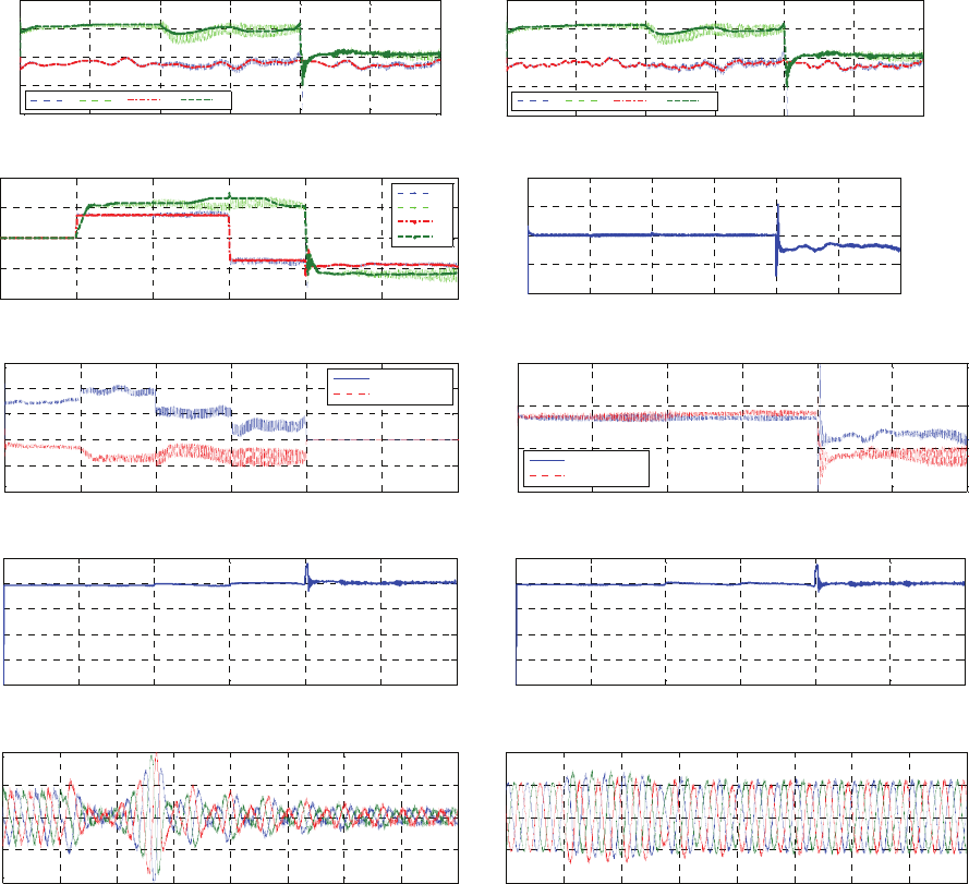
Fig. 7 shows the performance of the microgrid in
the grid-connected mode, islanding mode, and
transition from the grid-tied to islanding mode. Due
to variable weather conditions, the power transferred
from a wind turbine or solar array changed
constantly. This is represented by a changing d-axis
current as shown in Figs. 7a and 7b. Before t=2sec,
only wind and solar DERs at Bus 6 were connected
to the microgrid. At t=2sec, the battery at Bus 4was
connected to the microgrid with full charging power,
which increased the power supplied by the grid to
the microgrid (Fig. 7e). At t=4sec, non-critical loads
within the microgrid were curtailed to prepare for
the islanding operation, which increased voltage
distortion within the microgrid network as
demonstrated by higher d- and q-axis current
oscillation from wind, solar, and battery DERs in
Figs. 7a to 7c. At t=6sec, the battery shifted from
charge mode to discharge mode, which decreased
the power supplied by the grid even more (Fig. 7e).
During the grid-connected mode, the microgrid
frequency was stable (Fig. 7d) so that the reference
power of the battery converter depended mainly on
the charge or discharge power command from the
MGCC (Fig. 7c). At t=8sec, the microgrid shifted
from the grid-tied mode to the islanding mode.
Therefore, no power was transferred from the grid to
the microgrid after t=8sec (Fig. 7e) and at the same
time there was a large increase of the power supplied
by the microturbine (Fig. 7f). Note that in Figs. 7e
and 7f, the motor sign convention is used to represent
the power absorbed by the microgrid from the grid or
power absorbed by the microturbine from the
distribution network. In the islanding mode, the
microgrid frequency was more sensitive to the load
and DER power variations (Fig. 7d). The frequency
alteration caused the battery controller to adjust the
MGCC power reference according to the droop
principle (Eq. (22) and Fig. 7c). During both the
grid-tied and islanding modes, the microgrid voltage
was properly maintained around the desired value
(Figs. 7g and 7h). Although there was a high
oscillation in DER currents during the transition
from the grid-tied to islanding mode (Fig. 7i), the
current oscillation of the loads within the microgrid
is not obvious (Fig. 7j).
For each DER, only information about the
nominal PCC voltage, nominal dc voltage, and
resistance and inductance values of the grid filter is
required to train the neural network controller of the
DER converter. The same information is needed for
the design of a conventional controller, as well. After
the training, the neural network controller can be
applied to the DER converters in a microgrid,
although the distribution system structure seen by
each DER may be different. Again, the study shown
Control of Three-Phase Grid-Connected Microgrids using Artificial Neural Networks
65

by Fig. 7 demonstrates a great performance and
stability of the microgrid in grid-tied mode,
islanding mode, and transition from the grid-tied to
islanding mode by using the proposed neural
network vector controllers, which is an important
issue in microgrid operation (Bottrell et al., 2013;
Lee et al., 2013; Rowe et al., 2013).
6 CONCLUSIONS
This paper presented a neural network control
mechanism for the control of a microgrid and the
distributed energy sources within the microgrid. This
controller, which implements dynamic
programming, was trained with a
Levenberg-Marquardt backpropagation algorithm.
Compared to conventional vector control methods,
the neural network controller demonstrated a
stronger ability to determine optimal control actions
from multiple inputs. It boasts very fast response and
close to ideal controller performance. It does not
require synchronization to initially connect a DER or
a microgrdi to the grid, making it a potential solution
to many challenges in the operation and
management of DERs and future smart microgrids.
Using a neural network control technique, a
microgrid can achieve a better voltage profile, high
power quality and quick connection or disconnection
of a distributed energy source to the microgrid. In
future work, we plan to build a micro-scale
microgrid system and obtain real data and more
solid experiment results.
REFERENCES
S. N. Balakrishnan and V. Biega, Adaptive-critic-based
neural networks for aircraft optimal control, J.
Guidance, Control, and Dynamics, 19: 4, pp. 893–898,
1996.
R. E. Bellman, Dynamic Programming. Princeton, NJ:
Princeton Univ. Press, 1957.
F. Blaabjerg, R. Teodorescu, M. Liserre, and A. V.
Timbus, Overview of control and grid synchronization
for distributed power generation systems, IEEE Trans.
Ind. Electron., 53: 5, pp. 1398–1409, 2006.
N. Bottrell, M. Prodanovic, and T. C. Green, Dynamic
stability of a microgrid with an active load, IEEE
Trans. Power Electron., 28: 11, pp. 5107-5119, 2013.
S.-K. Chung, A phase tracking system for three phase
utility interface inverters, IEEE Trans. Power
Electron., 15: 3, pp. 431–438, 2000.
G. F. Franklin, J. D. Powell, M. L. Workman, Digital
Control of Dynamic Systems, Addison-Wesley, 1998.
R. Gagnon, Detailed Model of a Doubly-Fed Induction
Generator (DFIG) Driven by a Wind Turbine,The
MathWork, 2009.
M. T. Hagan, H. B. Demuth, and M. H. Beale, Neural
Network Design, Boston: PWS, 2002.
H. He, N. Zhen, and F. Jian, A three-network architecture
for on-line learning and optimization based on
adaptive dynamic programming, Neurocomputing, 78:
1, pp. 3-13, 2012.
F. Katiraei, R. Iravani, N. Hatziargyriou, and A. Dimeas,
Microgrid management, IEEE Power and Energy
Magazine, 6: 3, 2008, pp. 54-65.
C. Lee, C. Chu, and P. Cheng, A new droop control
method for the autonomous operation of distributed
energy resource interface converters, IEEE Trans.
Power Electron., 28: 4, pp. 1980-1993, 2013.
S. Li, M. Fairbank, C. Johnson, D. C. Wunsch and E.
Alonso, Artificial neural networks for control of a
grid-connected rectifier/inverter under disturbance,
dynamic and power converter switching conditions,
IEEE Trans. on NeuralNet. and Learning Systems, 25:
4, pp. 738–750, 2014.
S. Li, T.A. Haskew, Y. Hong, and L. Xu, Direct-current
vector control of three-phase grid-connected
rectifier-inverter, Electric Power System Research, 81:
2, 2011, pp. 357-366.
N. Mohan, T. M. Undeland, and W. P. Robbins, Power
Electronics: Converters, Applications, and Design,
3rd ed., John Wiley & Sons Inc., 2002.
S. Papathanassiou, N. Hatziargyriou, and K. Strunz, A
benchmark low voltage microgrid network, Proc. of
CIGRE Symposium: Power Systems with Dispersed
Generation, April 2005, Athens, Greece.
W. H. Press, B. P. Flannery, S. A. Teukolsky, and W. T.
Vetterling, Numerical recipes in C: The art of
scientific computing (second edition), Cambridge
University Press, 1992, pp. 994.
J. Rocabert, G. M. S. Azevedo, A. Luna, J. M. Guerrero, J.
I. Candela, and P. Rodríguez, Intelligent connection
agent for three-phase grid-connected microgrids, IEEE
Trans. on Power Electronics, 26: 10, 2011, pp.
2993-3005.
P. Rodríguez, A. Luna, R. S. Muñoz-Aguilar, I.
Etxeberria-Otadui, R. Teodorescu, and F. Blaabjerg, A
stationary reference frame grid synchronization system
for three-phase grid-connected power converters under
adverse grid conditions, IEEE Trans. Power Electron.,
27: 1, pp. 99–112, 2012.
C. N. Rowe, T. J. Summers, R. E. Betz, D. J. Cornforth,
and T. G. Moore, Arctan power–frequency droop for
improved microgrid stability, IEEE Trans. Power
Electron., 28: 8, pp. 3747-3759, 2013.
F. Y. Wang, H. Zhang, and D. Liu, Adaptive dynamic
programming: An introduction, IEEE Comput. Intell.
Mag., pp. 39–47, 2009.
NCTA 2015 - 7th International Conference on Neural Computation Theory and Applications
66
APPENDIX
a) Active and reactive power (neural network)
b) Active and reactive power (conventional)
c) Three-phase current (neural network)
d) Three-phase current (conventional)
Figure 1: Performance of PQ-inverter DER using conventional and neural network controllers (T
s
=1ms).
a) Active and reactive power (neural network)
b) Active and reactive power (conventional)
c) PCC voltage (neural network) d) PCC voltage (conventional)
Figure 2: Performance of PV-inverter DER using conventional and neural network controllers (T
s
=1ms).
a) Active and reactive power (neural network)
b) Active and reactive power (conventional)
Figure 3: PQ-inverter DER with constraints using conventional and neural network controllers.
0 1 2 3 4 5 6
-150
-100
-50
0
50
100
Power (kW /kVar)
Time (sec)
Active
Reactive
0 1 2 3 4 5 6
-150
-100
-50
0
50
100
Power (kW/kVar)
Time (sec )
Active
Reac tive
1.95 1.975 2 2.025 2.05
-200
-100
0
100
200
abc currents (A)
Time (sec )
1.95 1.975 2 2.025 2.05
-200
-100
0
100
200
abc currents (A)
Time (sec )
0 1 2 3 4 5 6
-150
-100
-50
0
50
100
Power (kW/kVar)
Time (sec )
Active Reac tive
0 1 2 3 4 5 6
-150
-100
-50
0
50
100
Power (kW/kVar)
Time (sec)
Active Reactive
0 1 2 3 4 5
350
375
400
425
450
Voltage (V)
Time (sec )
0 1 2 3 4 5
350
375
400
425
450
V
o
lt
age
(V)
Time (sec )
0 1 2 3 4 5 6 7
-150
-100
-50
0
50
100
Power (kW/kVar)
Time (sec )
P* Q* P Q
0 1 2 3 4 5 6 7
-200
0
200
400
Power (kW/kVar)
Time (sec )
P*
Q*
P
Q
Control of Three-Phase Grid-Connected Microgrids using Artificial Neural Networks
67
a) Active and reactive power (neural network) b) Active and reactive power (conventional)
c) PCC voltage (neural network)
d) PCC voltage (conventional)
Figure 4: PV-inverter with constraints using conventional and neural network controllers.
a) DER1 current (neural network)
b) DER1 current (conventional)
c) DER2 current (neural network)
d) DER2 current (conventional)
Figure 6: Three-phase currents when connecting DERs to the grid without synchronization control.
0 1 2 3 4 5 6 7
-200
-150
-100
-50
0
50
100
Power (kW/kVar)
Time (sec )
Active Reac tive
0 1 2 3 4 5 6 7
-200
0
200
400
Power (kW/kVar)
Time (sec )
Active
Reactive
0 1 2 3 4 5 6
350
375
400
425
450
Voltage (V)
Time (sec )
0 1 2 3 4 5 6 7
300
350
400
450
Voltage
(
V
)
Time (sec )
0.95 1 1.05 1.1 1.15 1.2
-300
-200
-100
0
100
200
300
a
b
c currents
(A )
Time (sec )
0.95 1 1.05 1.1 1.15 1.2
-300
-200
-100
0
100
200
300
a
b
c currents
(A )
Time (sec )
1.95 2 2.05 2.1 2.15 2.2 2.25 2.32.3
-400
-200
0
200
400
abc currents (A)
Time (sec )
1.95 2 2.05 2.1 2.15 2.2 2.25 2.32.3
-400
-200
0
200
400
a
b
c curren
t
s
(A )
Time (sec )
NCTA 2015 - 7th International Conference on Neural Computation Theory and Applications
68
a) Solar inverter d- and q-axis currents
b) Wind turbine inverter d- and q-axis currents
c) Battery inverter d- and q-axis currents
d) Microgrid frequency
e) Active and reactive power absorbed from the grid f) Active and reactive power of the microturbine
g) RMS line voltage at Bus 4 h) RMS line voltage at Bus 6
i) Three-phase PCC current of wind DER j) Three-phase load current at Bus 8
Figure 7: Performance of neural network controlled microgrid.
0 2 4 6 8 10 12
-200
-100
0
100
200
Currents (A)
Time (sec)
Id Iq Id* Iq*
0 2 4 6 8 10 12
-200
-100
0
100
200
C
urrents
(A)
Time (sec )
Id Iq Id* Iq*
0 2 4 6 8 10 12
-200
-100
0
100
200
Currents (A)
Time
(
sec
)
Id
Iq
Id*
Iq*
0 2 4 6 8 10 12
59
59.5
60
60.5
61
Frequency (Hz)
Time (sec )
0 2 4 6 8 10 12
-200
-100
0
100
200
300
Power (kW/kVar)
Time (sec )
Active power
Reac tive power
0 2 4 6 8 10 12
-200
-100
0
100
Power (kW/kVar)
Time (sec )
Active power
Reactive power
0 2 4 6 8 10 12
0
100
200
300
400
500
Voltage (V)
Time (sec )
0 2 4 6 8 10 12
0
100
200
300
400
500
Voltage (V)
Time (sec )
7.95 8 8.05 8.1 8.15 8.2 8.25 8.3 8.35
-200
-100
0
100
200
Current (A)
Time (sec )
7.95 8 8.05 8.1 8.15 8.2 8.25 8.3 8.35
-100
-50
0
50
100
Current (A)
Time (sec )
Control of Three-Phase Grid-Connected Microgrids using Artificial Neural Networks
69
