Road Estimation and Fuel Optimal Control of an Off-Road Vehicle

orgen Albrektsson

1,2

and Jan

Aslund

Department of Electrical Engineering, Link

oping University, SE-581 83 Link

oping, Sweden

Volvo Construction Equipment, SE-631 85 Eskilstuna, Sweden

Keywords:

Off-road, Construction Equipment, Kalman Filters, Rolling Resistance, Optimal Control, Dynamic Program-

ming.

Abstract:

This paper explores the possibility to use optimal control to establish a Pareto front of fuel consumption vs

cycle time for a transport mission with an articulated hauler. The Pareto front can be utilised to optimise the

hauler transport mission on its own or as a part in a larger optimal control problem involving several con-

struction machines working together on a site transporting material at a set production rate. While rolling

resistance is a major energy consumer in an articulated hauler’s transport, the effect of varying rolling re-

sistance is included in the developed optimisation algorithm. A method utilising Extended Kalman Filter,

Rauch-Tung-Striebel smoothing and sensor fusion is formulated in order to calculate the road related data

needed in the optimisation algorithm. A potential fuel efﬁciency improvement, veriﬁed by computer simula-

tions, of up to 9% was found in the example transport mission where the optimal gear and speed trajectory

were followed instead of driving towards a mean speed target to achieve an equal cycle time for the transport

mission.

1 INTRODUCTION

In the construction industry today articulated haulers

are used in a vast amount of different transport mis-

sions due to its ability to work efﬁciently even at

tough (off-)road conditions. Commonly there is a set

production target [ton/h] for the transport mission, i.e.

the hauler should transport a certain amount of mate-

rial in a set time. This work explores the possibility

to use optimal control to establish a Pareto front of

fuel consumption vs cycle time for a transport mis-

sion with an articulated hauler. The Pareto front can

be utilised to optimise the transport mission on its

own or as a part in a larger optimal control problem

involving several construction machines. Predictive

cruise control is today a common feature in commer-

cial vehicles. Through calculation of an optimal ve-

hicle speed trajectory on a priori known road stretch

a reduction in fuel consumption and CO

emissions

can be achieved. The optimisation algorithm anal-

yses the road elevation to make use of the potential

energy that is released in down slopes, preserves the

energy as kinetic energy in the vehicle which is then

used when the road is going up again. In combina-

tion with optimising the choice of gear, enabling the

internal combustion engine (ICE) to work efﬁciently,

further fuel consumption reduction is possible. The

working conditions of an off-road vehicle differ in

some respects substantially compared to an on-road

vehicle. Off-road the ﬂuctuation in elevation of the

road is steeper and more frequent and the road sur-

face is much rougher. The differences in the working

environment results in a much lower average speed

of an off-road vehicle compared to an on-road truck.

These conditions shifts the relation between energy

consumers making rolling resistance dominate over

air-drag off-road compared to the opposite in a typi-

cal on-road truck application (21st Century truck part-

nership, 2013). In (Fu and Bortolin, 2012) the possi-

bility of using Dynamic Programming is explored to

optimise a vehicle speed trajectory and to build a gear

shift strategy for an articulated hauler. This paper ex-

pands earlier research through also consider varying

rolling resistance in the optimisation algorithm and to

include an algorithm that estimates the rolling resis-

tance along the track. The paper is disposed as fol-

lows: Section 2 presents a vehicle model of an ar-

ticulated hauler, the model is essentially equal when

applied both in the map module and optimisation al-

gorithm. In Section 3 a method to estimate and record

the road characteristics is developed. Section 4 dis-

plays a method for optimal control of the hauler and

the method used to build the Pareto front. Section 5

presents results from tests and simulations.

Albrektsson, J. and Åslund, J.

Road Estimation and Fuel Optimal Control of an Off-Road Vehicle.

DOI: 10.5220/0006247200580067

In Proceedings of the 3rd International Conference on Vehicle Technology and Intelligent Transport Systems (VEHITS 2017), pages 58-67

ISBN: 978-989-758-242-4

2 VEHICLE MODEL

In this section the driveline and the complete vehicle

are modelled. The models are used both in the map

module and in the optimisation algorithm. The dis-

played models are the ones used in the map module

while the end of the section explains the needed up-

dates when applied in the optimisation algorithm.

2.1 External Forces Acting on the

Hauler

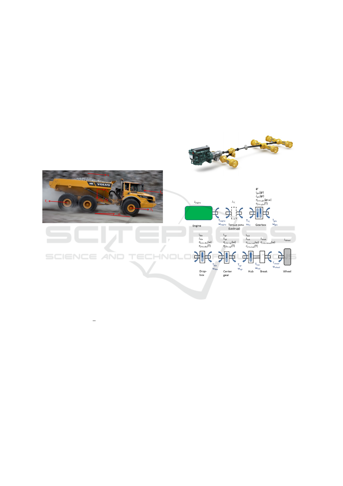
There are several forces acting on a vehicle as it starts

to move, see i.e. (Guzzella and Sciaretta, 2013).

The main longitudinal forces acting on the articulated

hauler are displayed in Figure 1.

Figure 1: Longitudinal forces acting on an articulated

hauler.

In Figure 1 the following models / notation apply:

Vehicle Speed, v

Road Inclination, α

Tractive Force (retarding if negative), F

Aerodynamic Force, F

. The motion of an object

through the atmosphere gives rise to an aerodynamic

resisting force. For a vehicle F

is often modelled to

be dependent on the density of the surrounding air,

, the front area of the vehicle, A

, an aerodynamic

drag coefﬁcient, c

and the velocity of the vehicle, v,

in square.

· A

· c

· v

(1)

Rolling Resistance Force, F

. The rolling resistance

force can be modelled as

= c

· m

veh

· g ·cos(α) (2)

The rolling resistance coefﬁcient, c

, depends on

many variables such as vehicle speed, tire pressure

and road surface conditions. In our case the rolling

resistance coefﬁcient is one of the parameters that are

estimated in the map building process and variations

in these variables will indirectly affect the estimation

of c

Force Generated by Road Inclination, F

. As the

vehicle moves up-hill or down-hill the gravity will

create a retarding or accelerating force depending on

the angle of the slope, α. This force is modelled as

= m

veh

· g · sin(α) (3)

2.2 Drivetrain Model

The drivetrain in a Volvo articulated hauler is shown

in Figure 2. The main components in the hauler driv-

etrain are from left to right: internal combustion en-

gine, torque converter, gear box, drop box, central

gear, hub, brake and (wheel).

Figure 2: Drivetrain in a Volvo A40G Articulated hauler.

Figure 3: Drivetrain model.

Figure 3 displays how the model of the drivetrain

is built. The notation used in picture 3 is: T = torque

[Nm], ω = angular velocity [rad/s], gr = gear [-], J =

mass moment of inertia [ kgm

], i = gear ratio [-], η

= efﬁciency [ % ].

Internal Combustion Engine ( ICE ). When

used in the map module the measured torque gen-

erated by the internal combustion engine is an input

to the drivetrain model. The net generated torque,

engine

, is estimated by the engine management sys-

tem (EMS) and broadcasted on the vehicle CAN net-

work. No deeper description on how the torque is es-

timated by the EMS is considered to be needed at this

point. Newton’s second law of motion, with dots rep-

resenting the time derivatives, connects angular accel-

eration to torque,

engine

= T

engine

− T

(4)

where J = inertia, ω

engine

= engine angular speed and

is the torque at node torque converter.

Road Estimation and Fuel Optimal Control of an Off-Road Vehicle

Torque Converter ( TC ). A torque converter

with lock-up functionality is bolted on the crankshaft

of the ICE connecting the engine to the gear box. A

Volvo A40G hauler is predominantly running in lock-

up mode. Only at take-off and at very steep uphill

slopes the hauler runs in torque converter mode. Thus

the drivetrain model is limited to only consider lock-

up mode and the TC is modelled as a stiff axle with

additional inertia according to (5):

= T

engine

= ω

engine

(5)

Gear Box ( gbx ). The Volvo A40G is equipped

with a Powertronic gear box with 9 forward gears and

4 reverse gears. The Powertronic gearbox is of plan-

etary type and gear shifts are made by means of en-

gaging and disengaging clutches. A major advantage

with this design is that gear shifts can be performed

without torque loss and the vehicle loses no kinetic

energy during a gear shift. During the gear shift a

change in efﬁciency of the gear box is likely but this

is not reﬂected in the gear box model when used in

the map module since it is judged to be of minor im-

portance when estimating the road grade. In the gear-

box there are three types of efﬁciency losses: friction,

viscous and a loss stemming from an oil pump in the

gearbox. The friction coefﬁcient, µ

gbx

is gear depen-

dent and derived from measurements. The speed and

gear dependency of the viscous loss is interpolated

from measured curves. The loss from the oil pump

is modelled as a constant. The model of the gearbox

becomes:

gbx. f ric

= T

· i

gbx

(gr) · µ

f ric

(gr)

gbx



− T

gbx.pump



· i

gbx

(gr) −

gbx.visc

(ω

,gr)| − |T

gbx. f ric

(6)

gbx

engine

gbx

(gr)

(7)

Drop Box ( dbx ). The dropbox is a gear box

placed in the middle of the hauler translating the

power downwards in the vehicles vertical direction

and splitting it to the front axle and rear axles. Sim-

ilar to the gearbox a friction loss and a viscous loss

applies. Equation (8) to (9) displays the model of the

drop box.

dbx. f ric

= (T

gbx

· i

dbx

− |T

dbx.visc



gbx



|) · µ

f ric

dbx

= T

gbx

· i

dbx

− |T

dbx.visc



gbx



| − |T

dbx. f ric

(8)

dbx

gbx

dbx

(9)

Centre Gear ( cgr ). The denomination centre

gear is used for the differential gear in the middle of

the axle. The centre gear is modelled as:

cgr. f ric

= T

dbx

· µ

f ric

cgr

= (T

dbx

− |T

cgr. f ric

|) · i

cgr

− |T

cgr.visc

(10)

cgr

dbx

cgr

(11)

Hub Reduction ( hub ). In the hub of the wheel

a reduction gear and the brake is placed. The hub

reduction gear is modelled according to the equations

below.

hub. f ric

= T

cgr

· µ

f ric

hub

= (T

cgr

− |T

hub. f ric

|) · i

hub

− |T

hub.visc

(ω

cgr

(12)

hub

cgr

hub

(13)

Wheel Brake ( brake ).

The wheel brake is mounted in the hub. A speed

dependent viscous loss applies to the brake indepen-

dent if the wheel brakes are applied or not. If the

wheel brakes are in operation the hydraulic brake

pressure is measured and broadcasted via CAN. The

wheel brake is modelled according to (14) to (16),

brake

= P

brake

· A

brakepiston

· µ

brake

(ω

hub

)

· N

f ric.disc

· r

f ric.disc

(14)

wheel

= T

hub

− |T

break.visc

(ω

hub

)| − T

brake

(15)

wheel

= ω

hub

(16)

where P

brake

= brake pressure, A

brakepiston

= area of

brake piston, µ

brake

= speed dependent brake disc fric-

tion coefﬁcient, N

f ric.disc

= number of brake friction

discs and r

f ric.disc

= average brake friction disc radius.

A threshold is set to the brake pressure to avoid mea-

surement ripple, thus, when P

brake

≤ 200kPa, T

brake

set to 0.

Wheels ( Wheel ). At the wheels the torque gen-

erated by the ICE and the applied brake force is trans-

lated into a traction (or retardation) force, F

, see

equation (17). At the wheels, the rotational inertia is

also translated into a equivalent mass, equation (18),

wheel

(17)

rot.TC

= (J

engine

+ J

gbx−in

)

· (i

gbx

(gr) · i

dbx

· i

cgr

· i

hub

)

wheel

rot.gbx

= (J

gbx−out

+ J

dbx−in

)

· (i

dbx

· i

cgr

· i

hub

)

wheel

rot.dbx

= (J

dbx−out

+ J

cgr−in

) · (i

cgr

· i

hub

)

wheel

rot.cgr

= (J

cgr−out

+ J

hub−in

) · (i

hub

)

wheel

rot.wheel

= (J

hub−out

+ J

brake

+ J

wheel

)/r

wheel

(18)

where r

wheel

is the radius of the wheel. The equivalent

rotational mass is summarised with the vehicle mass,

veh

, to a total mass denominated m

tot

= m

veh

+ m

rot.TC

+ m

rot.gbx

+ m

rot.dbx

+ m

rot.cgr

+ m

rot.wheel

(19)

VEHITS 2017 - 3rd International Conference on Vehicle Technology and Intelligent Transport Systems

2.3 Complete Vehicle Model

Combining the drivetrain model, the external forces

and Newton’s second law of motion enables an ex-

pression for the longitudinal dynamics of the hauler.

In continuous time the expression is:

tot

(gr) ·

v(t) = F

(t)−F

(t) (20)

where gr = gear and t = time.

2.4 Model Alteration for Optimisation

The complete vehicle model is to a large extent reused

when applied in the optimal control algorithm. Fol-

lowing the energy ﬂow with the aim to calculate the

engine speed and torque corresponding to a step in

position and states, the structure of Section 2.1 to 2.3

is reused but in reversed order. When the ICE speed

and torque is known it is translated into a fuel ﬂow.

Wheel Brake and Hub Reduction

(torque/speed node cgr). Differing from the

wheel brake model in Section 2.2 there is no need to

calculate the brake force when calculating the fuel

cost. If the step in energy state (speed decrease)

is negative and large enough so that application of

the wheel brakes is necessary to achieve balance in

equation (42), this will render in a loss of kinetic

energy but since the ICE will operate without adding

positive torque, no fuel will be injected and thus the

fuel cost is 0.

Torque Converter and Auxiliary Equipment

(torque/speed node engine). As the torque converter

is modelled only to be operating in lock-up mode, the

hauler never comes to full stop and consequently the

energy state is always > 0 in the optimised speed tra-

jectory. In practise this has limited impact since the

very high combined gear ratio in a hauler enables very

low vehicle speeds and since it is only at the end of

the cycle v = 0 is desired. At the engine speed/torque

node the loss from the ICE’s auxiliary equipment (al-

ternator, fan, etc) is added by means of a look-up ta-

ble, equation (21). This is not necessary when the

model is used for road estimation since the measured

torque signal from the engine ECU includes the aux-

iliary equipment loss.

Engine

= T

+ T

aux.equip

(ω

) (21)

Internal Combustion Engine (ICE). The inter-

nal combustion engine model in the optimisation al-

gorithm consists of a measured look up table with en-

gine speed, ω

Engine

, and engine torque, T

Engine

as in-

put and the fuel mass ﬂow, ˙m

as output. The cost in

fuel mass, m

[kg], for one step in distance with corre-

sponding changes of states is evaluated using equation

(45).

3 ESTIMATION OF ROAD

INCLINATION AND ROLLING

RESISTANCE

Section 3 outlines a method for collecting the road re-

lated data that is needed in the optimisation algorithm.

The intention is to use sensors available in a standard

articulated hauler complemented with a commercially

available GPS. The data is collected and processed in

a Matlab algorithm and the road is stored in a map

like format with latitude and longitude coordinates as

identiﬁcation points. The main parameters that are

identiﬁed in the algorithm are: latitude (ϕ), longitude

(λ), altitude (z), mean vehicle speed (v), road incli-

nation (α), vehicle heading (β), rolling resistance co-

efﬁcient (c

), speed limit (v

max

) and travelling direc-

tion (Dir.). Of the quantities stored in the map, only

ϕ,λ,α,c

and v

max

are used in the optimisation algo-

rithm presented in Section 4. A method to estimate

the road inclination for on-road commercial vehicles

is exhaustively described in (Sahlholm, 2011) and has

been further enhanced for off-road vehicles and to in-

clude rolling resistance in the work of (Almes

aker,

2010) and (Saaf and Hana, 2011). The method used

utilizes an extended Kalman ﬁlter (EKF) to work as

an observer for the unmeasured parameter rolling re-

sistance and also to help removing potential bias error

that develops when only using an inclination sensor to

measure the road inclination (Sahlholm, 2011), p.80-

88. In the estimation model, Section 3.2.6, the vehicle

model described in Section 2 and the road model de-

scribed in Section 3.2.5 are combined to generate the

quantities stored in the road map.

3.1 Map Building Process

The intention with the proposed map building process

is that the operator initially travels the track between

the loading and unloading sites 2 times to initiate the

map. The map data is updated off-line after each ﬁn-

ished run which is a feasible scenario on a construc-

tion site since the distance between the loading and

unloading sites normally are within 2 km (approx. 6

min travel). On a high level, the map building process

can be described according to the steps below:

1. Operator drives the track between the loading and

unloading site forth and back as fast (but safe) as

possible while necessary sensor data is recorded.

2. The direction of the travel is detected and the data

updated accordingly.

3. The collected data is processed in the map-

building algorithm according to:

(a) Calculation of applied brake force.

Road Estimation and Fuel Optimal Control of an Off-Road Vehicle

(b) Translation of ICE torque into force at wheels.

sured and calculated) are merged in an Ex-

tended Kalman Filter (EKF).

(d) Smoothing of estimates with Rauch-Tung-

Striebel algorithm to remove potential lag.

(e) Merge the estimates into a map utilising a fu-

sion algorithm.

4. The highest recorded speed at each coordinate is

used to set the max speed limit.

As additional runs are travelled during production

new data is merged into the map after each run, im-

proving the quality of the map.

3.2 Sensor and Data Fusion

The proposed map building algorithm utilises data

recorded from an external GPS: ϕ, λ,z,β and the vehi-

cle CAN: v, α, vehicle articulation (Φ), engine torque

engine

). The GPS sensor used in the tests was a

Garmin GPS18x OEM. The accuracy according to the

manufacturer (Garmin international inc., 2011) is for

position: < 15m, 95 % typical and for velocity: 0.1

knot RMS steady state in GPS Standard Positioning

Service mode and position: < 3m, 95 % typical and

velocity: 0.1 knot RMS steady state in WAAS mode.

No speciﬁc data on the accuracy of the altitude signal

is given.

3.2.1 Time vs Spatial Sampling

The predominant way to describe a road is through

map coordinates. Using distance rather than time as

the independent variable facilitates the fusion of data

from several different runs along the road since dif-

ferent runs may have been travelled in opposing di-

rection and at different speeds. To shift to distance as

the independent variable the following conversion is

used in the vehicle’s longitudinal model.

= v

⇒

,v 6= 0 (22)

3.2.2 Sensor Fusion

Several different methods for sensor fusion are avail-

able, see e.g. (Gustafsson, 2012). The Kalman ﬁlter

and the extended Kalman ﬁlter (EKF) are well-known

mathematical methods for sensor fusion that also en-

ables the possibility to estimate the states of a pro-

cess. This is a valuable feature since the rolling re-

sistance is not directly measurable with the standard

mounted sensors on an articulated hauler. While the

Kalman ﬁlter method only are able to estimate the

states of a linear process the extended Kalman ﬁlter

method gives the possibility to estimate the states in a

non-linear process (Welch and Bishop, 2006). Based

on the ﬁndings in (Sahlholm, 2011) and (Almes

aker,

2010) the extended Kalman ﬁlter was chosen as the

method for sensor fusion in the map building pro-

cess. The use of the extended Kalman ﬁlter in the

proposed map building process follows to a large ex-

tent the guidance given in (Welch and Bishop, 2006).

3.2.3 Smoothing

To compensate for ﬁltering delay and to include later

measurements in the estimate for each data point a

smoother is applied after each run. The Rauch-Tung-

Striebel (RTS) smoother (Rauch et al., 1965) is an ef-

ﬁcient two-pass algorithm for ﬁxed interval smooth-

ing. The use of the RTS smoother is possible since

the intention is to update the map only after a com-

plete run along the road.

3.2.4 Data Fusion

A general data fusion method is used to merge data

from different runs along the road. The data fusion

method is described in (Gustafsson, 2012), p.30. Af-

ter the data has been merged, the data is stored in the

map for each coordinate pair along with the covari-

ance matrix.

3.2.5 Road Model

In the proposed road model the identiﬁcation points

are separated with a nominal distance ∆s, as described

in Section 3.2.7. Out of the 7 appended road pa-

rameters only the correlation between road altitude,

z, and road inclination angle, α, is modelled as the

other parameters are either measured or observed in

the Kalman ﬁlter. The correlation between road alti-

tude and road inclination angle is modelled as

= sin(α(s)) (23)

3.2.6 Estimation Model

This section describes how the road parameter esti-

mation is made and the models used in the estimation

process.

Extended Kalman Filter ( EKF ) and Smoothing.

The states to be estimated presented in continuous

time are displayed in (24).

ˆx (t) = [ϕ(t) λ(t) z (t) v (t) α (t) β(t) c

(t)]

(24)

VEHITS 2017 - 3rd International Conference on Vehicle Technology and Intelligent Transport Systems

The explanation of the parameters are found in the

beginning of this section. As described in 3.2.1 spa-

tial samples are used instead of continuous time in the

model. To shift to distance as the independent vari-

able equation (22) is used. Equation (24) is translated

into discrete notation, see equation (25), where k rep-

resents the index of the location.

ˆx

= [ϕ

r.k

]

(25)

Time update (a priori estimate).

1. Deﬁne two distances, one in meters and one in

degrees:

∆s

m.k

= ˆv

· T

∆s

deg.k

∆s

m.k

earth

180

(26)

2. Project the state ahead (state equations).

ˆx

−







k−1

+ ∆s

deg.k−1

cos(α

k−1

)cos(β

k−1

)

k−1

+ ∆s

deg.k−1

cos(α

k−1

)sin(β

k−1

)

k−1

+ ∆s

m.k−1

sin(α

k−1

)

k−1

∆s

m.k−1

k−1

t.k−1

−F

a.k−1

−F

g.k−1

−F

r.k−1

tot

k−1

+ ∆s

m.k−1

cos(α.k−1)

turn.k−1

r.k−1







(27)

With:

turn.k−1

= l

cot(Φ

k−1

) +

sin(Φ

k−1

)

(28)

where r

turn

is the turning radius of the vehicle, Φ is the

articulation angle, l

and l

distances between axles

and articulation point (front / rear).

3. Project the error covariance ahead

Deﬁne the Jacobian: A[i,j] = df[i]/dx[j] and

project the error covariance:

−

= A · P

k−1

· A

+ Q (29)

4. Measurement update (a priori estimate) Deﬁne

the measurement vector:



k.gps

k.CAN

k.gps



(30)

Measurement equation:

= H · x

+ e

(31)

where the H matrix is:

H =



∗7

= 0



(32)

Calculate the Kalman gain:

= P

−

(HP

−

+ R)

−1

(33)

5. Update estimates with measurement

ˆx

= ˆx

−

+ K

− H ˆx

−

) (34)

6. Update error covariance

= (I − K

H)P

−

(35)

7. Save ˆx

, P

, ˆx

−

and P

−

at each coordinate [k]

to be used in smoothing process.

8. Initiate smoothing with the last predicted val-

ues ( ˆx

−

N+1|N

) and last predicted covariance matrix

−

N+1|N

), where N is the total number of measured

data points. Run smoothing backwards along the

track. Kalman smoothing gain:

= P

k|k

+ A

−−1

k+1|k

(36)

Smoothed estimates:

ˆx

k|N

= ˆx

k|k

+ K

( ˆx

k+1|N

− ˆx

−

k+1|k

) (37)

Smoothed error covariance matrix

k|N

= P

k|k

k+1|N

− P

−

k+1|k

(38)

3.2.7 Fusion of Map Data

A reference track is chosen and split into 6m long

sections. The knot points are identiﬁed through the

ϕ and λ coordinates and the corresponding states are

appended. When the reference map is compared with

a recorded track the search area of new measurements

is limited to points which have the same heading,

≤ 15

◦

and to a rectangular area that is ±1.5m in the

heading direction and ±8m orthogonal to the heading.

If driven in reversed direction, the sign of α and the

heading is switched (180 deg). Out of the points in

the new track that is in the search area, the point that

is closest to the reference point in the horizontal plane

is chosen. The tracks are merged into the stored map

through fusion of independent estimates as described

in (Gustafsson, 2012), p.30. The states in the map is

calculated according to equation (39).

= ((P

)

−1

+ (P

)

−1

)

−1

ˆx

= P

· ((P

)

−1

ˆx

+ (P

)

−1

ˆx

)

(39)

4 OPTIMAL CONTROL OF AN

ARTICULATED HAULER

In this section a method to control the velocity and

gear shift of an articulated hauler as it travels along a

road with varying inclination and surface conditions

is developed. The target is to derive a Pareto front

of minimum fuel consumption vs cycle time. Input

to the optimisation algorithm is machine data and the

road dependent data developed in Section 3.

Road Estimation and Fuel Optimal Control of an Off-Road Vehicle

4.1 Objective

The objective is to transport material at a set produc-

tion rate [ton/hour], which easily translates into cycle

time, while minimising fuel consumption. A Pareto

front is built through running the optimisation proce-

dure a number of times with different cycle time tar-

gets achieving a set of discrete cycle time - min fuel

consumption points. Denominating each individual

optimisation procedure with i, the objective becomes:

minimise M

i = 1, ...,n (P1)

s.t. t

where M

= fuel consumption in cycle i and t

= cy-

cle time in cycle i. Dynamic programming is used as

method for the optimisation and to avoid the Curse

of dimensionality ((Bellman, 1961)) the approach of

(Monastyrsky and Golownykh, 1993) and (Hellstr

et al., 2010) is used, i.e. the trip time is added to the

criteria in (P1) which becomes:

minimise M

+ β

t i = 1, ...,n (P2)

The trade-off between fuel consumption and cycle

time is represented by the scalar coefﬁcient β. The n

number of discrete points in the Pareto front is estab-

lished through varying β n times. The lower limit of

the cycle time in the Pareto front is found through set-

ting β high enough to reach maximum speed limit and

the upper limit is found through setting β low enough

so no further fuel consumption decrease is found.

4.2 Dynamic Programming

Dynamic Programming (DP), developed in the 1950’s

by Richard Bellman, is a well known algorithm to

solve optimal control problems. Considering road

topology and rolling resistance as a priori known dis-

turbances (by means of the earlier described map-

module) and since dimension is small, DP suits the

optimal control problem at hand well. While the DP

algorithm is not described in-depth here, the reader

is referred to (Bellman and Dreyfus, 1962) and e.g.

(Guzzella and Sciaretta, 2013).

4.2.1 State Space

While it is the cycle time / fuel consumption trade off

that is the main objective a natural choice for the ﬁrst

state variable would be vehicle speed. However, fol-

lowing the ﬁndings in (Hellstr

om et al., 2010), hav-

ing energy as the state variable damps the oscilla-

tory behaviour of the control while using the preferred

Euler forward method for discretisation. Thus, en-

ergy is chosen as the ﬁrst state variable. The sec-

ond state variable is gear number rendering in the

state vector: x

= [ e

]

, where e = energy and

gr = gear number. Denominating the control vari-

ables u, the control vector is u



e.k

gr.k



[ e

k+1

− e

k+1

− gr

]

4.2.2 Control Constraints

Since the proposed drivetrain model is limited to lock-

up mode, see Section 2.4, a min limit for the velocity

needs to be set. The max limit of the speed is an input

to the optimisation procedure from the map module.

Consequently the vehicle speed is limited to

min

≤ v ≤ v

max

(40)

Due to limitations in the gearbox a limit on gear

steps is introduced i.e. the maximal number of gear

shifts is 2 (both up and down shift).

− 2 ≤ gr

k+1

≤ gr

+ 2 (41)

4.3 Dynamic Model

The vehicle model in Section 2, with alterations de-

scribed in Section 2.4, is used. Thus the complete

vehicle model is the same as in equation (20). Trans-

lated into spatial coordinates and reformulated into

terms of energy (20) becomes:

= F

− F

(42)

4.4 Discretisation

The optimisation problem is solved numerically and

must be discretised. The data from the map module

is discrete and split into N steps of length h such that

the total distance of the transport mission, S, equals

S =

∑

k=1

(43)

Utilising Euler forward method to discretise equa-

tion (42), the discretised complete vehicle model is

written

k+1

− e

= F

t.k

− F

a.k

− F

r.k

− F

g.k

(44)

Similarly the fuel mass ﬂow ˙m

is transformed

into spatial representation using equation (22) and

then discretised with the Euler method.

f .k+1

= m

f .k

˙m

f .k

(45)

VEHITS 2017 - 3rd International Conference on Vehicle Technology and Intelligent Transport Systems

4.5 Cost Function

The cost function is a central part of the DP algo-

rithm and in the work at hand based on calculating the

equivalent fuel cost, m

, for bringing the vehicle from

one position on the road to the next position. Dur-

ing the transition both states, i.e. the kinetic energy

(speed) and the gear, may change. A time penalty, in-

troduced in Section 4.1 and the cost for changing gear

described below, are added to the cost function.

ζ = m

+ βt + m

f .gs

(46)

Differing from the drivetrain model in the map

module, see 2.2, the efﬁciency loss in the gearbox at

gear shifts is accounted for in the optimisation algo-

rithm. The cost of a gear shift is approximately equal

to the work that is lost speeding up or slowing down

the engine to meet the next gear. In the model, this is

implemented as the fuel ﬂow needed to accelerate or

decelerate the engine inertia plus the inertia of com-

ponents up to the point where the gear is engaged.

The fuel ﬂow is multiplied with the time of the gear

shift resulting in a fuel mass penalty, m

f .gs





engine.k

(gr) − ω

engine.k+1

(gr)





(47)

∗ J (48)

f .gs

= ˙m

f .gs

(ω

engine.k

) · t

(49)

5 RESULT

To test the map module a 1.2km long gravel road

was travelled with an articulated hauler 3 times in

each direction while needed sensor data was recorded.

The data was processed off-line in a Matlab script

designed according to the method described in Sec-

tion 3. A comparison between measured / estimated

parameters and the resulting fusioned data stored in

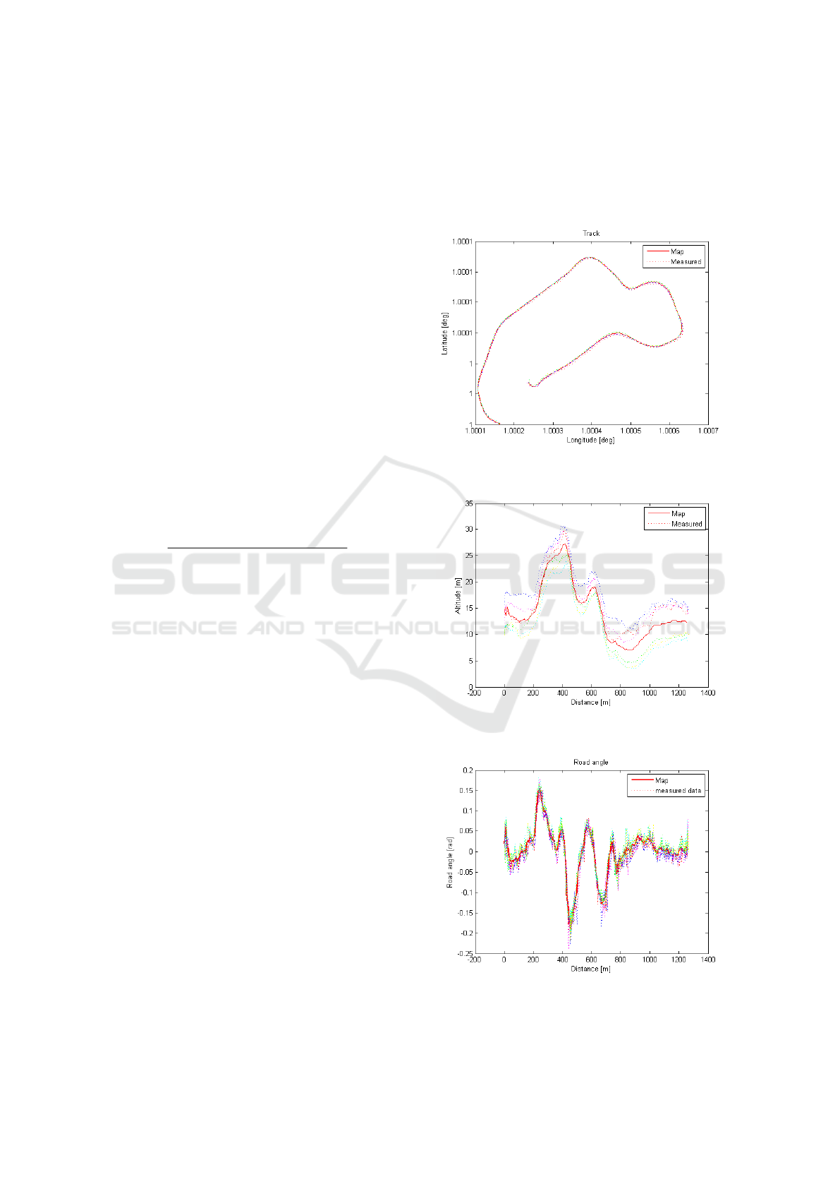
the map is shown in Figure 4 to 7. As seen in Fig-

ure 4 and 5 the latitude - longitude and especially the

altitude signal from the GPS have rather poor accu-

racy. In the vertical plane the spread in the GPS sig-

nal is approximately 10m. Also the signal from the

road angle sensor is wildly ﬂuctuating in real working

condition. Except for the endpoints of the track, the

use of sensor fusion and fusion of data from several

runs averages the spread in the individual measure-

ments to make a uniform estimation of the road. At

the endpoints of the track (i.e. the loading/unloading

area) there is much larger spread in the hauler’s move-

ments (position, speed, heading, articulation etc.) and

the method has some difﬁculties in ﬁnding reference

measurements rendering in some unexpected ﬂuctua-

tion in the stored map. A solution to this would be

to deﬁne a loading respectively unloading area, e.g.

implemented as a circle, and then only store map data

between the periphery of the two circles.

Figure 4: Measured and resulting latitude and longitude

coordinates stored in the map. (axes normalised)

Figure 5: Measured and resulting altitude stored in the

map.

Figure 6: Measured and resulting road angle stored in the

map.

Road Estimation and Fuel Optimal Control of an Off-Road Vehicle

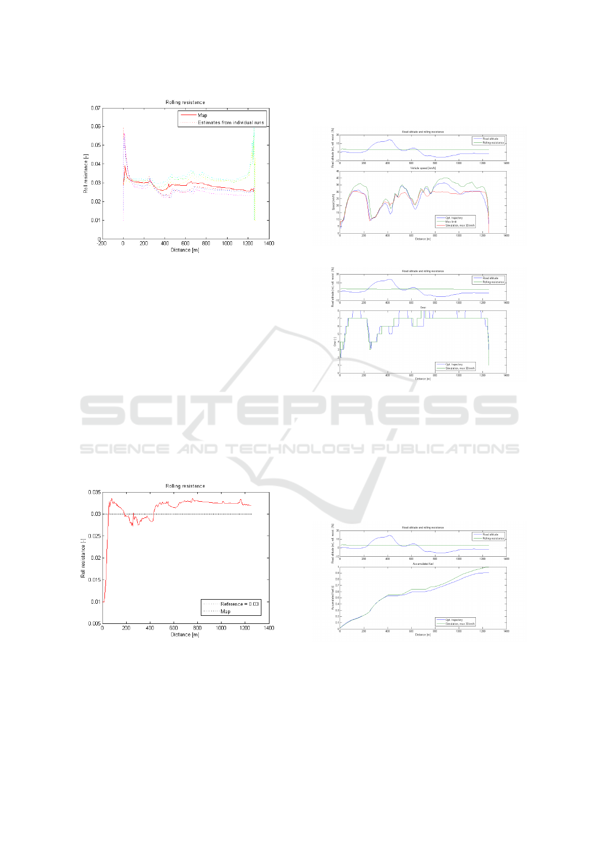
Figure 7: Individual estimations and fusioned rolling

resistance stored in the map.

A test to see how well the method estimates the

rolling resistance was performed. Since it is very

difﬁcult to measure the rolling resistance of an ar-

ticulated hauler in actual working conditions, the

measured GPS data was combined with a pre-set

rolling resistance, c

= 3%, and then the hauler drive

was simulated with a Volvo in-house developed soft-

ware to generate the engine torque and speed signals

needed in the map module. The map module was run

on the created data and a comparison of the estimated

rolling resistance and the pre-set is shown in Figure 8.

Even if only one drive is used as input, due to difﬁ-

culties in syncing measured and simulated data, (the

estimation is enhanced if several turns are driven) the

rolling resistance is well represented after some ini-

tialisation time.

Figure 8: Veriﬁcation of rolling resistance estimation.

Utilising the created map as input to the opti-

mal control module a speed and gear shift optimisa-

tion can be performed. Figure 9 to 10 displays op-

timal speed and gear-shift trajectories when the time

penalty is set to β = 0.007g/s. In the ﬁgures a com-

parison is made to speed and gear trajectories as sim-

ulated with an in-house Volvo tool when the speed is

limited to 30/km/h which gives a similar cycle time.

Figure 9: Vehicle speed trajectory.

Figure 10: Gear trajectory.

As seen in Figure 9 in the optimal trajectory the

hauler picks-up speed in the down slopes generating

kinetic energy which is utilised when the road goes

up. Figure 10 shows that when the gear shift is opti-

mised higher gear is consistently used enabling lower

engine speeds and reducing fuel consumption. The

combination of optimal speed and gear saves approx.

9 % fuel compared to when a ﬁxed target speed is set.

The comparison of how the fuel consumption devel-

ops along the track is shown in Figure 11.

Figure 11: Accumulated fuel consumption (normalised).

Following the method described in Section 4.1 a

Pareto front trading fuel consumption against cycle

time is built, see Figure 12. The graph shows a clear

increase in fuel consumption if the cycle time is de-

creased below approx. 200s.

VEHITS 2017 - 3rd International Conference on Vehicle Technology and Intelligent Transport Systems

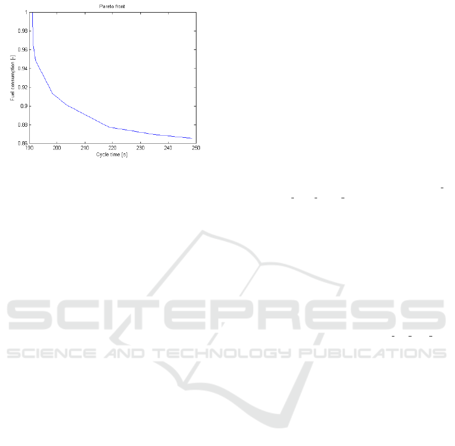
Figure 12: Pareto front showing trade-off (normalised) fuel

consumption vs cycle time.

6 CONCLUSION

A method to generate a map which includes parame-

ters important for optimisation in off-road conditions,

such as road inclination and rolling resistance, has

been developed. The method utilises sensors mounted

as standard on a Volvo articulated hauler combined

with a commercially available GPS sensor. The main

algorithms used is an extended Kalman ﬁlter to merge

sensors, a RTS smoother to remove the ﬁlter lag and

a data fusion algorithm to merge data from several

runs along the road. The map is used as input to the

optimal control problem to minimise fuel consump-

tion in a articulated hauler transport mission towards

a set cycle time. A Dynamic Programming algorithm

is developed to solve the optimal control problem.

In the DP algorithm, optimal vehicle speed and gear

shift trajectories are computed enabling the hauler to

make best use of its kinetic energy and to consistently

choose high gears to enable low engine speed, min-

imising fuel consumption. In the test case, a poten-

tial reduction of fuel consumption of up to 9%, ver-

iﬁed by computer simulations, is shown when com-

pared to a simulation of the same transport mission

where a ﬁxed mean speed target is used to achieve an

equal cycle time. The proposed optimisation method

is utilised to create a Pareto front of fuel consump-

tion vs cycle time for the transport mission, which can

be used for the hauler transport itself or when solv-

ing a larger optimal control problem involving several

construction machines working together on a trans-

port mission. Different means to get the articulated

hauler to follow the optimal control trajectories are

plausible. One is to implement a human machine in-

terface (HMI) instructing the driver to follow the op-

timal speed trajectory, a second could be to design a

cruise control software that controls speed and gear

shifts (under the operators supervision) and in an au-

tonomous hauler the system could be integrated into

the control system of the machine.

ACKNOWLEDGEMENTS

This research is supported by FFI - Strategic Vehicle

Research and Innovation.

REFERENCES

21st Century truck partnership (2013). 21st cen-

tury truck partnership and technical white papers.

www.energy.gov/sites/prod/ﬁles/2014/02/f8/21ctp

roadmap white papers 2013.pdf.

Almes

aker, B. (2010). Iterative map building for gear shift

decision. Master’s thesis, Uppsala University.

Bellman, R. (1961). Adaptive control process. Princeton

University Press.

Bellman, R. E. and Dreyfus, S. E. (1962). Applied dynamic

programming. Princeton University Press.

Fu, J. and Bortolin, G. (2012). Gear shift optimization

for off-road construction vehicles. In Procedia - so-

cial and behavioral science, volume 54. SCIENCEDI-

RECT.

Garmin international inc. (2011). Gps

18x technical speciﬁcations.

http://static.garmin.com/pumac/GPS 18x Tech

Specs.pdf.

Gustafsson, F. (2012). Statistical sensor fusion. Studentlit-

teratur AB, 2:1 edition.

Guzzella, L. and Sciaretta, A. (2013). Vehicle propulsion

systems. Springer-Verlag, 3 edition.

Hellstr

om, E.,

Aslund, J., and Nielsen, L. (2010). Design

of an efﬁcient algorithm for fuel-optimal look-ahead

control. Control Engineering Practice, 18(11):1318–

1327.

Monastyrsky, V. V. and Golownykh, I. M. (1993). Rapid

computations of optimal control for vehicles. Trans-

portation Research, 27B(3):219–227.

Rauch, H. E., Striebel, C. T., and Tung, F. (1965). Maxi-

mum likelihood estimates of linear dynamic systems.

AIAA Journal, 3(8):1445–1450.

Saaf, M. and Hana, A. (2011). Map building and gear shift

optimization for articulated haulers. Master’s thesis,

alardalen University.

Sahlholm, P. (2011). Distributed road grade estimation for

heavy duty vehicles. PhD thesis, Royal Institute of

Technology, Stockholm.

Welch, G. and Bishop, G. (2006). An introduction to the

kalman ﬁlter. Technical report, University of North

Carolina at Chapel Hill.

Road Estimation and Fuel Optimal Control of an Off-Road Vehicle