
Spikiness Assessment of Term Occurrences in Microblogs:
An Approach based on Computational Stigmergy
Mario G. C. A. Cimino
1
, Federico Galatolo
1
, Alessandro Lazzeri
1
,
Witold Pedrycz
2
and Gigliola Vaglini
1
1
Department of Information Engineering, University of Pisa, Largo Lazzarino 1, Pisa, Italy
2
Department of Electrical and Computer Engineering, University of Alberta, Edmonton, T6R 2V4 AB, Canada
mario.cimino@unipi.it, f.galatolo1@studenti.unipi.it, alessandro.lazzeri@for.unipi.it,
wpedrycz@ualberta.ca, gigliola.vaglini@unipi.it
Keywords: Microblog Analytics, Spikiness Assessment, Computational Stigmergy, Term Cloud.
Abstract: A significant phenomenon in microblogging is that certain occurrences of terms self-produce increasing
mentions in the unfolding event. In contrast, other terms manifest a spike for each moment of interest,
resulting in a wake-up-and-sleep dynamic. Since spike morphology and background vary widely between
events, to detect spikes in microblogs is a challenge. Another way is to detect the spikiness feature rather
than spikes. We present an approach which detects and aggregates spikiness contributions by combination
of spike patterns, called archetypes. The soft similarity between each archetype and the time series of term
occurrences is based on computational stigmergy, a bio-inspired scalar and temporal aggregation of
samples. Archetypes are arranged into an architectural module called Stigmergic Receptive Field (SRF).
The final spikiness indicator is computed through linear combination of SRFs, whose weights are
determined with the Least Square Error minimization on a spikiness training set. The structural parameters
of the SRFs are instead determined with the Differential Evolution algorithm, minimizing the error on a
training set of archetypal series. Experimental studies have generated a spikiness indicator in a real-world
scenario. The indicator has enhanced a cloud representation of social discussion topics, where the more
spiky cloud terms are more blurred.
1 INTRODUCTION
Microblogging systems are increasingly used in the
everyday life, producing in real time a huge amount
of informal and unstructured messages. In the
literature, a research challenge is to identify and
separate the temporal dynamics of a specific event,
summarizing or visualizing such information in
order to make it accessible to human analysts. A
relevant dynamic is that certain occurrences of terms
self-produce increasing mentions in the unfolding
event, whereas other terms manifest a spike for each
moment of interest, resulting in a wake-up-and-sleep
pattern called spikiness (Gruhl & Guha, 2004),
(Highfield et al., 2013).
Automatic spike detection on Microblogs is a
difficult task, because: (i) experts usually provide
simplistic spike definitions; (ii) two human experts
often do not mark the same events as spikes; (iii) the
ratio of candidate spike events to actual spike events
is large; (iv) spike morphology and background vary
widely between events; (v) well defined training set
are time consuming and expensive to develop.
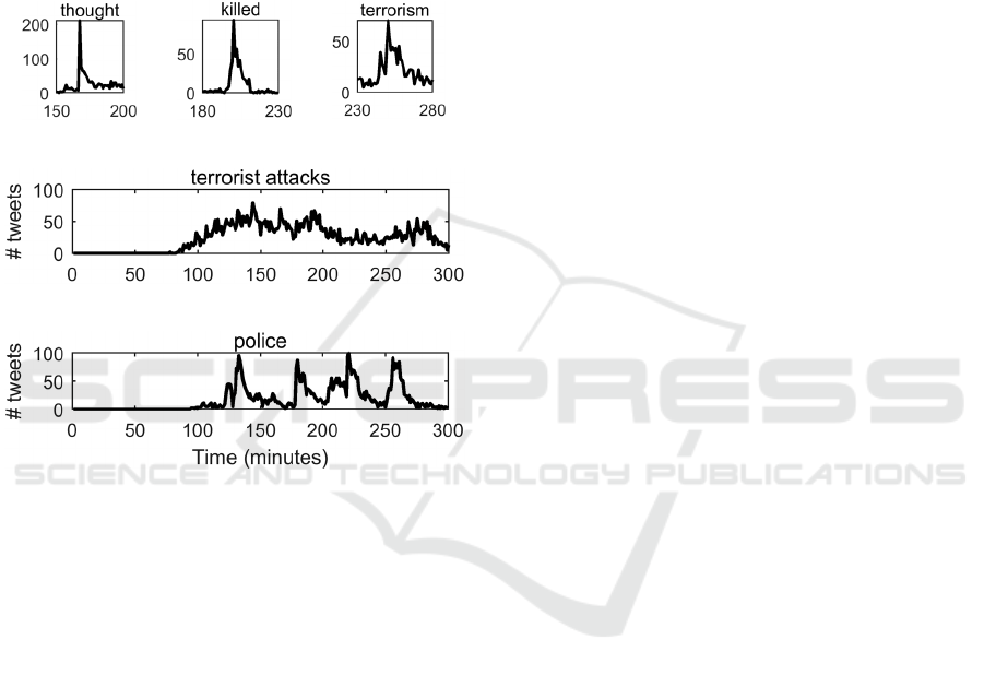
As an example, Fig. 1 shows the dynamics of
some major terms used on Twitter during the
terrorist attack in Paris on 13 Nov 2015, by gunmen
and suicide bombers. In particular, Fig. 1a-c show
different spike morphologies and durations: thought
(short duration), killed (medium duration), and
terrorism (long duration). Fig. 1d-e show different
spikiness degrees: terrorist attack (low spikiness)
and police (high spikiness).
In the literature, many statistical and machine
learning techniques have been used for the automatic
spike detection (Yun, 2011), (Marcus et al., 2011),
(Nichols et al., 2012), (Lehmann et al., 2012),
(Birdsey et al., 2015). In this paper we present an
innovative technique based on computational
stigmergy (Avvenuti, 2013), (Barsocchi, 2015), a
bio-inspired paradigm of emergent systems. In the
literature, a well-known form of stigmergy is
manifested by by societies of insects (Dorigo et al.
2000), (Mohan et al. 2012).
In the basic mechanism of stigmergic computing
Cimino, M., Galatolo, F., Lazzeri, A., Pedrycz, W. and Vaglini, G.
Spikiness Assessment of Term Occurrences in Microblogs: An Approach based on Computational Stigmergy.
DOI: 10.5220/0006253807310737
In Proceedings of the 6th International Conference on Pattern Recognition Applications and Methods (ICPRAM 2017), pages 731-737
ISBN: 978-989-758-222-6
Copyright
c
2017 by SCITEPRESS – Science and Technology Publications, Lda. All rights reserved
731
each sample of a time series releases a mark (i.e. a
digital pheromone) in the scalar space, evaporating
over time. As a result, marks with scalar and
temporal proximity overlap, generating functional
structures called trails. A trail enables a short-term
and short-size granulation mechanism, appearing
and staying spontaneous at runtime when local
dynamics in samples occurs. A similarity operator is
used to associate the dynamic of a sequence of
samples against a collection of predefined sequences
called archetypes.
(a) (b) (c)
(d)
(e)
Figure 1: Three spikes morphologies and durations: (a)
short spike duration, (b) medium spike duration, (c) long
spike duration. Two spikiness degrees: (d) low spikiness,
(e) high spikiness.
The computational unit of our architecture is
called Stigmergic Receptive Field (SRF) (Cimino et
al. 2006). We use SRFs to detect the spikiness of
time series generated by event-specific terms. In a
SRF, the spikiness feature is modeled by a collection
of archetypal spikes with different morphologies.
The training of a SRF consists in optimizing its
parameters via the Differential Evolution algorithm
(Cimino et al. 2015), (Alfeo et al., 2016). The SRF
compares the stigmergic trail released by an
archetypal spike with the stigmergic trail of the
current time series, and provides the measure of
similarity. To combine the different spikiness
morphology represented by the different archetypal
spikes, the SRFs are arranged in a Stigmergic
Perceptron (SP). Since the SP manages archetypal
spikes of a specific scale, multiple SPs have been
used to identify different sized spikiness. Finally, the
spikiness indicator is generated through a linear
combination of SRFs, whose weights are calculated
by means of the Least Square Error minimization on
some desired spikiness provided by human experts.
The paper is structured as follow: Section 2
summarizes the related works on spike detection in
Microblogs. Section 3 comprises the design of the
functional modules of our approach. Section 4
covers the experimental studies. Finally, Section 5
draws conclusions and future work.
2 RELATED WORK
Several authors studied the dynamics of temporal
usage of terms in Microblogs, using distance
measures for time series (Fu 2011), (Esling et al.,
2012). Gruhl & Guha (2004) present three main
types of topics pattern on blogs: (i) just spike: topics
which at some point switch from inactive to very
active, and then back to inactive; (ii) spiky chatter:
topics with a significant chatter level, very sensitive
to external world events; (iii) mostly chatter, topics
continuously discussed at relatively moderate levels.
Highfield et al. (2013) examine the use of Twitter
for the expression of shared fandom in the context of
the Eurovision Song Contest. The authors found that
the presence of a spike is usually related to particular
event occurred during the show.
Yun (2011) distinguishes between three types of
topic: peaky topics, constant topics and regularly
repeated topics. The author defines specific criteria
and uses statistical methods to differentiate the three
categories. Marcus et al. (2011) identify spikes in a
temporal collection of tweet, by computing the
average rate of messages in a sliding window. More
precisely, a spike is found when the rate in a window
is a local maximum, i.e. the side windows have
lower rates. Nichols et al. (2012) present an
algorithm for spike detection used to summarize
sporting events from Twitter messages. The
algorithm is based on the change in the volume of
the published tweet per minute according to a slope
threshold. The threshold is computed for the entire
event from basic statistics of the set of all slopes for
that event. Similarly, Lehmann et al., (2012) study
the daily evolution of hashtags popularity over
multiple days, considering one hour as a time unit.
The identification of an activity peak is based on the
change in the volume according to a statistical
baseline and a tunable threshold. They identify four
different categories of spike-shaped temporal
patterns, depending on the concentration around the
event: before and during the event, during and after
ICPRAM 2017 - 6th International Conference on Pattern Recognition Applications and Methods
732

the event, symmetrically around the event, and only
during the event. Birdsey et al. (2015) propose an
approach based on four state of a topic: rising,
plateau, burst, and stabilization. To identify the state
the authors define a metric named intensity, which is
directly proportional to the number of messages
related to the topic and the number of total users
(publishers), and inversely proportional to the total
number of messages and the number of unique user
posting on the topic. According to a threshold and
the metric, the topic switches from a state to another.
3 FUNCTIONAL DESIGN
This Section formally introduces the major
functional components of our algorithm.
3.1 The Stigmergic Receptive Field
Let
() denote the values of a time series at
discrete-time k. A linear transformation of the time
series called min-max normalization is assumed:
()
( ) MinMaxNorm( ( ))
M
IN
M
AX MIN
dk d
dk dk
dd
−
=
−
(1)
which is a linear mapping of the data samples in the
interval [0,1], where the bounds
and
are
estimated in an observation time window. To assure
samples are positioned between 0 and 1, the results
are clipped to [0,1].
Normalized data samples are processed by
clumping, in which samples of a particular range
group close to one another. Clumping is a kind of
parametric soft discretization of the continuous-
valued samples to a set of levels:
2
2
( ) Clumping( ( ); , )
0, ( )
()
2, ()
2
()
12 , ()
2
1, ( )
CCC
c
ccc
c
cc
ccc
c
cc
c
dk dk
dk
dk
dk
dk
dk
dk
αβ
α
αα
β
α
βα
βαβ
β
βα
β
≡
≤
−+
<≤
−
−+
−<<
−
≥
(2)
As an implementation of clumping, we adopt the
s-shaped function, shown in Fig. 2a. Given
,(0,1)
CC
α
β
∈ input values smaller | larger than (β
C
– α
C
)/2 are lowered | raised; values smaller | larger
than α
C
| β
C
assume the minimum | maximum value,
i.e., 0|1. Fig. 2b shows an example of series, in
dotted line, and the effect of the clumping, in solid
line.
Clumped data samples are processed by
marking, in which each sample produces a
corresponding mark:
12
() Marking( (); , )
C
Mk d k
εε
≡
(3)
As an implementation of marking, we adopt the
trapezoid function, shown in Fig. 3, defined by the
center
()
C
dk
, a fixed height equals to 1, upper and
lower-bases, ε
1
and ε
2.
Since the ratio ε
1
/ε
2
is
statically prefixed to 2/3, we can refer to the mark as
Marking( ( ); )
C
dk
ε
.
(a) (b)
Figure 2: The s-shaped function with 0.22
c
α
= and
0.76
c
β
= (a), and the clumping (solid) of the input series
(dotted).
Figure 3: The trapezoidal mark, centered in
0.5
c
d =
,
with
1
0.4
ε
=
and
2
0.6
ε
=
.
With the trailing, the evaporation and the
accumulation of the marks over time create the trail
structure:
( ) Trailing( ( 1), ( ); )Tk Tk Mk
δ
≡−
(4)
0, ( 1)
()
(1) ,
if T k
Tk
T k otherwise
δ
δ
−≤
′
=
−−
(5)
() () ()Tk T k Mk
′
=+
(6)
The evaporation is regulated by the rate
01
δ
≤<
. Fig. 4a and Fig. 4a show the release of a
mark with
2
0.24
ε
=
on
(0) 0
c
d =
, and the trail after
the evaporation with
0.34
δ
=
and the release of the
second mark on
(1) 0
c
d =
.
Spikiness Assessment of Term Occurrences in Microblogs: An Approach based on Computational Stigmergy
733

(a) (b)
Figure 4: (a) The release of a mark with ε
2
= 0.24 on d
C
(0)
= 0; (b) The trail after the evaporation with
0.34
δ
=
and
the release of the second mark on d
C
(1) = 0.
As a consequence, an isolated mark tends to
disappear from the trail, reducing the influence of
spurious samples in the temporal pattern. In contrast,
subsequent marks sum their intensities if
superimposed with other marks generating a more
persistent structure.
A Stigmergic Receptive Field (SRF) is fed by
two time series, i.e.,
()dk
and
()dk
. Given a
sliding time window, of size N, it takes two parallel
segments
{()}
N
dk ≡
1
{ ( ),..., ( )}
N
dk dk
{()}
N
dk ≡
and
1
{ ( ),..., ( )}
N
dk dk
, and returns the activation
() [0,1]ah∈
, which is close to 0 | 1 if the two
segments are dissimilar | similar. As an example Fig.
5 shows two input parallel segments, with N=25.
(a) (b)
Figure 5: Two input segments (a)
{()}dk
and (b)
{()}dk
of a Stigmergic Receptive Field.
In a SRF, the two segments are processed in
parallel, by means of clumping, marking and
trailing, thus generating two corresponding trails
()Tk and
()Tk
. Subsequently, the similarity
between the two trails is computed:
( ) Similarity( ( ), ( )) [0,1]sh Tk T k≡∈
(7)
As an implementation of similarity, we adopt the
Jaccard’s coefficient, which is the ratio between the
intersection and the union of the trails:
() () () () ()
s
hTkTkTkTk∩∪
(8)
As an example, Fig. 6 shows two trails (in solid
and dotted line), the intersection (dark gray), and the
union as the area covered by the light gray, dark
gray, and the white areas underlying the trails.
Figure 6: Representation of the intersection and union
between two trails.
We remark that for each pair of segment, each
made by N samples, a single similarity sample s(h)
is released, i.e.
/Nkh= , 1N .
Finally, the activation of the similarity sample is
computed:
() Activation((); , )
AA
ah sh
α
β
≡
(9)
As an implementation of activation, we adopt the
s-shaped function. The activation increases |
decreases the rate of similarity potential firing the
SRF. The term “activation” is borrower from neural
sciences: it inhibits low intensity signals while
boosts signals reaching a certain level to enable the
next layer of processing (Cimino, 2009).
We remark that, although the clumping and the
activation are implemented by the same function,
their meaning is very different. Indeed, in contrast to
the activation, the clumping may be implemented by
a multi-level s-shape function, when different levels
of interest are comprised in the input space.
3.2 The Adaptation of the SRF
The SRF should be properly parameterized to enable
an effective aggregation of input samples and output
activation:
()
()
{()} ,{()} ; , ,, , ,
CC AA
N
N
ah
SRF d k d k
α
β
εδα
β
=
(10)
For example, short-life marks evaporate too fast,
preventing aggregation and pattern reinforcement,
whereas long-life marks cause early activation.
The adaptation is an offline function, taking as
an input a SRF and a tuning set made by a set Z of
(input, desired output) pairs. As an output, the
adaptation provides a set of structural parameters of
the SRF:
{
}
(
)
Adaptation ,{(*), (*)} , (*)
{, ,,, , }
N
cc aa
SRF d k d k a h
αβεδαβ
=
(11)
As an implementation of adaptation, we use the
Differential Evolution algorithm. In (Cimino, 2015),
ICPRAM 2017 - 6th International Conference on Pattern Recognition Applications and Methods
734
the authors carry out a comparative study of three
evolutionary algorithms: Particle Swarm Optimiza-
tion, Genetic Algorithm, and Differential Evolution.
As a result, the latter shows better performance both
in speed and quality of the solution. The fitness
function is the Mean Squared Error (MSE) between
the output SRF' provided for a certain input and the
desired output SRF provided in the tuning set for the
same input:
()
2
1
()
zz
z
fZ SRF SRF
Z
′
=−
(12)
The objective is to train the SRF to accurately
recognize the (dis-)similarity between segments.
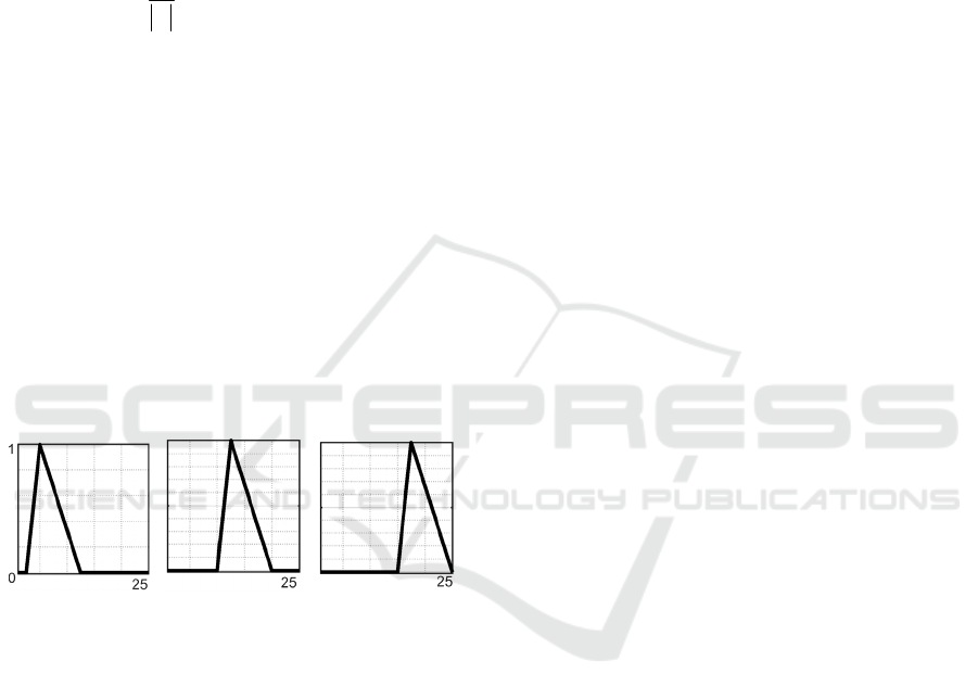
3.3 The Stigmergic Perceptron
A single SRF can be used to recognize the (dis-)
similarity between a time series and an archetypal
time series, which represents a pattern. In the
spikiness domain, we can have more than one
archetype. Fig.7 shows three spikiness archetypes in
a time window. Here, the different positions of the
archetypes represent an early, a timely, and a late
spike. This allows identifying the spike independen-
tly on the temporal shift with respect to the time
window.
(a) (b) (c)
Figure 7: Spikiness archetypes: (a) early spike; (b) timely
spike; (c) late spike.
A Stigmergic Perceptron takes as an input the
output of each SRF, one per each archetype, and
provides the output of the SRF with the best
activation:
{
}
() SP ()
g
hSRFh≡
(13)
As an implementation of the SP, we use the
maximum between the activations:
{
}
() max ()
SRF SRF
g
hah
(14)
3.4 The Spikiness Information Fusion
The assessment of the spikiness level of the overall
series is based on the aggregation of three different
Stigmergic Perceptrons. Each SP employs different
archetypes: short spike duration, medium spike
duration, and long spike duration. The assessment is
based on a number of U non-overlapping time
windows, for each SP. The outputs of each SP are
summated:
1
()
U
iiu
u
ASPh
=
=
(15)
Given that there are no dependencies between the
processing of each SP, the values of A
i
can be
computed in parallel.
Finally, the activation values
k
A
are aggregated
by means of a weighted sum to generate the
spikiness level:
()
3
1
{};{}
L
EVEL i i i i
i
SSIFAw Aw
=
≡∗
(16)
the weights
i
w are determined through a standard
Least Square Error optimization, which minimizes
the error with respect to a set of spikiness level
generated by human observation:
()
*
Optimization { },{ } { }
L
EVEL i
SP S w=
(17)
It follows (Algorithm 1) the overall algorithm for
the calculation of the spikiness level of a set of given
time series {D}.
4 EXPERIMENTAL STUDIES
To study the effectiveness of the algorithm, we have
analyzed a dataset of 188,607 Twitter posts collected
during the terrorist attacks in Paris on November 13,
2015, between 9 PM of November 13 and 2 AM of
November 14.
The dataset was first pre-processed by removing
stop words, i.e., common words used in a language.
We also removed the historical baseline, i.e., a set of
terms generally related to the class of the event
rather than to its specific occurrence. Subsequently,
the most frequent 100 terms were selected, and the
corresponding time series were generated using a
time windows of 1 minute.
The time series were annotated by a group of
four human annotators, who assigned two different
indicators to each series:
(i) spikiness level: it is an integer ranging from 0
(no-spikiness) to 4 (maximum-spikiness). As an
example, the series of Fig.1d and Fig.1e have
spikiness levels 1 and 4, respectively. In general,
the spikiness level is proportional to the number
Spikiness Assessment of Term Occurrences in Microblogs: An Approach based on Computational Stigmergy
735

of occurrences of the wake-up-and-sleep
dynamic. The spikiness level is then normalized
dividing by 4.
(ii) spikiness dimension: it is the characterization of
the overall durations of spikes. Let us assume the
three types of spike represented in Fig.1 a-c, with
an order: 1: short, 2: medium, 3: high. Let us
consider the series of Fig.1e: since the medium
duration is the most frequent, and the short
duration is less frequent, the spikiness dimension
is 2|3|1. Considering Fig.1d, the short duration is
the most frequent, and the long duration is the
less frequent. Thus, the spikiness dimension is
1|2|3. Actually, the most wake-up-and-sleep
dynamics are not complete in Fig.1e, but our
focus is on spikiness rather than on spikes.
Algorithm 1: Spikiness ({
}).
D
← MinMaxNorm(
)
{
}
(
)
Adaptation ,{(*), (*)} , (*)
{, ,,, , }
N
cc aa
SRF d k d k a h
αβεδαβ
=
()
*
Optimization { },{ } { }
L
EVEL i
SP S w=
par for each d in {D}
par for each i in {SP}
par for each time window h
for each instant k
( ) Clumping( ( ); , )
CCC
dk dk
α
β
≡
( ) Marking( ( ); )
C
Mk d k
ε
≡
( ) Trailing( ( 1), ( ); )Tk Tk Mk
δ
≡−
end for
( ) Similarity( ( ), )
s
hTkT≡
() Activation((); , )
AA
ah sh
α
β
≡
{
}
() SP ()
g
hSRFh≡
end for
1
()
U
iiu
u
ASPh
=
=
end for
end for
()
{};{}
LEVEL i i
SSIFAw≡
return S
LEVE
L
Each annotator observed all the time series to
have an overview of the temporal patterns. Finally,
the annotators achieved consensus providing the
indicators for each time series.
Table 1 shows the confusion matrix of the human
classification compared with the same output
provided by the system. We remark that the 86% of
the time series are correctly identified by the system
(diagonal values, represented in boldface). A
significant number of misclassification is between
the dimensions 2|1|3 and 1|2|3, which means that
some spikes with short and medium duration are
inversely ranked.
The evaluation of the error on spikiness level is
calculated with a 5-fold cross-validation: we divided
our dataset into five randomly generated and
equally-sized folds. Then, we used each fold as a test
set and the remaining folds as a training set. Finally,
we calculated the average MSE± standard deviation,
as shown in Table 2. We remark that the MSE on the
training and test sets are very similar, thus
confirming the good generalization of the system.
We also remark that MSE is less than half of the
difference between two spikiness levels (1/4 = 0.25),
thus confirming a good accuracy. Finally, the
standard deviation is more than an order of
magnitude lower than the MSE, thus showing a good
precision.
Table 1: Confusion matrix of the spikiness dimension.
System
1|2|3
1
|
3
|
2
2
|
1
|
3
2
|
3
|
1
3
|
1
|
2
3
|
2
|
1
Human
1|2|3
21
0 4 0 0 0
1|3|2 0
4
2 0 0 0
2|1|3 2 0
53
1 0 0
2|3|1 1 0 3
7
0 0
3|1|2 0 0 0 0
1
1
3|2|1 0 0 0 0 0 0
Table 2: Fitness of the 5-Fold Cross Validation.
MSE (mean ± standard deviation)
Training Set Test Set
0.1146±0.0037 0.1197±0.0184
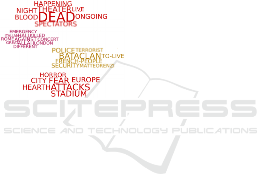
As a final result, the spikiness level has been
used to enrich the term cloud representing the
content of the discussion topics of a given event.
Fig.8 shows an excerpt of a term cloud with a blur
proportional to the spikiness level. Here, it is
apparent that even large terms can have a high
spikiness level, and those terms without spikiness
are clearly discerned.
5 CONCLUSIONS
This paper presents an innovative computational
technique for assessing the spikiness of terms in
microblogs. The core processing is based on
computational stigmergy, a bio-inspired mechanism
ICPRAM 2017 - 6th International Conference on Pattern Recognition Applications and Methods
736
for scalar and temporal processing of time series.
Experimental results have shown a very high
number of correctly detected spikiness dimension,
and a very low error on spikiness level for training
and testing sets. The spikiness indicator has been
visualized in a term cloud as a blur effect, making it
apparent. To conduct performance evaluations on
other datasets as well as comparative analyses with
other approaches is considered a key investigation
activity for future work.
Figure 8: An excerpt of the term cloud with blur
proportional to the spikiness level.
ACKNOWLEDGEMENTS
This work was partially supported by the PRA 2016
project “Analysis of Sensory Data: from Traditional
Sensors to Social Sensors” funded by the University
of Pisa.
REFERENCES
Alfeo, A. L., Appio, F. P., Cimino, M. G., Lazzeri, A.,
Martini, A., & Vaglini, G., 2016. An Adaptive
Stigmergy-based System for Evaluating Technological
Indicator Dynamics in the Context of Smart
Specialization. In ICPRAM 2016, 5th International
Conference on Pattern Recognition Applications and
Methods, INSTICC, pp. 497-502.
Avvenuti, M., Cesarini, D., Cimino, M.G.C.A., 2013.
MARS, a multi-agent system for assessing rowers'
coordination via motion-based stigmergy. Sensors,
MDPI, 13(9), 12218-12243.
Gruhl, D., Guha, R., 2004. Information Diffusion Through
Blogspace. In WWW’04, 13th International World
Wide Web Conference, pp. 491–501.
Highfield, T., Harrington, S., Bruns, A., 2013. Twitter as a
technology for audiencing and fandom. Information,
Communication & Society, Taylor & Francis, 16(3),
315-339.
Barsocchi, P., Cimino, M.G.C.A., Ferro, E., Lazzeri, A.,
Palumbo, F., Vaglini, G., 2015. Monitoring elderly
behavior via indoor position-based stigmergy.
Pervasive and Mobile Computing, Elsevier Science,
23, 26-42.
Birdsey, L., Szabo, C., Teo, Y. M., 2015. Twitter knows:
understanding the emergence of topics in social
networks. In WSC 2015, the 2015 Winter Simulation
Conference, IEEE, pp. 4009-4020.
Cimino, M.G.C.A., Pedrycz, W., Lazzerini, B.,
Marcelloni, F., 2009. Using Multilayer Perceptrons as
Receptive Fields in the Design of Neural Networks.
Neurocomputing, Elsevier Science, 72(10-12), 2536-
2548.
Cimino, M.G.C.A., Lazzeri, A., Vaglini, G., 2015.
Improving the analysis of context-aware information
via marker-based stigmergy and differential evolution,
In ICAISC 2015, International Conference on
Artificial Intelligence and Soft Computing, Springer
LNAI, Vol. 9120, Part II, pp. 1-12.
Dorigo, M., Bonabeau, E., Theraulaz, G.,2000. Ant
algorithms and stigmergy. Future Generation
Computer Systems, 16(8), 851-871.
Esling P., Agon, C. Time-series data mining, 2012, ACM
Computing Surveys, 45(1) 12.
Fu, T.C., A review on time series data mining, 2011,
Engineering Applications of Artificial Intelligence, 24,
164-181.
Lehmann, J., Gonçalves, B., Ramasco, J. J., Cattuto, C.,
2012. Dynamical classes of collective attention in
twitter. In WWW 2012, 21st international conference
on World Wide Web, ACM, pp. 251-260.
Marcus, A., Bernstein, M. S., Badar, O., Karger, D. R.,
Madden, S., Miller, R. C., 2011. Twitinfo: aggregating
and visualizing microblogs for event exploration. In
SIGCHI 2011, conference on Human factors in
computing systems, ACM, pp. 227-236.
Mohan, C.B., Baskaran, R., 2012. A survey: Ant Colony
Optimization based recent research and
implementation on several engineering domain.
Expert Systems with Applications, 39(4), 4618-4627.
Nichols, J., Mahmud, J., Drews, C., 2012. Summarizing
sporting events using twitter. In IUI 2012, the 2012
ACM international conference on Intelligent User
Interfaces, ACM, pp. 189-198.
Yun, H. W., 2011. Classifying temporal topics with
similar patterns on Twitter. Journal of information and
communication convergence engineering, 9(3), 295-
300.
Spikiness Assessment of Term Occurrences in Microblogs: An Approach based on Computational Stigmergy
737
