Anomaly Detection in Real-Time Gross Settlement Systems
Ron Triepels
1,3
, Hennie Daniels
1,2
and Ronald Heijmans
3
1
Tilburg University, Tilburg, The Netherlands
2
Erasmus University, Rotterdam, The Netherlands
3
De Nederlandsche Bank, Amsterdam, The Netherlands
Keywords:
Anomaly Detection, Neural Network, Autoencoder, Real-Time Gross Settlement System.
Abstract:
We discuss how an autoencoder can detect system-level anomalies in a real-time gross settlement system by
reconstructing a set of liquidity vectors. A liquidity vector is an aggregated representation of the underlying
payment network of a settlement system for a particular time interval. Furthermore, we evaluate the perfor-
mance of two autoencoders on real-world payment data extracted from the TARGET2 settlement system. We
do this by generating different types of artificial bank runs in the data and determining how the autoencoders
respond. Our experimental results show that the autoencoders are able to detect unexpected changes in the
liquidity flows between banks.
1 INTRODUCTION
Financial market infrastructures play a vital role in the
smooth functioning of the economy. They facilitate
the clearing and settlement of monetary and other fi-
nancial transactions. A particular type of system in
these infrastructures is the Real-Time Gross Settle-
ment (RTGS) system. An RTGS system is a system
that settles transactions of its participants individually
(gross) and immediately (real-time).
It is important to supervise the activities of banks
in financial systems. This is because financial sys-
tems tend to exhibit a robust-yet-fragile nature (Gai
and Kapadia, 2010). Banks may be well capable of
absorbing financial imbalances. However, if they start
experiencing liquidity issues, than these issues can
quickly propagate to many other banks due to their in-
terconnectedness. For this reason, much research has
recently been devoted to study the topology of pay-
ment networks and its impact on systemic risk. Sys-
temic risk is the risk associated with any event that
threatens the stability of a financial system as a whole
(Berndsen et al., 2016). It is commonly measured by
concepts of network theory, e.g. the centrality or de-
gree of a payment network.
In this paper, we present a different approach to
measure systemic risk. We apply anomaly detection
on the payment data generated by a RTGS system.
Generally, an anomaly is defined as a pattern that does
not conform to expected behavior (Chandola et al.,
2009). Accordingly, anomaly detection is the task of
automatically identifying anomalies in data. In our
case, anomalies are particular configurations of a pay-
ment network that deviate considerably from the ex-
pected norm. They are caused by financial stress or
unwanted payment behavior.
The application of anomaly detection on payment
data is promising. Payment data provide an accu-
rate and system-wide overview of how banks man-
age their liquidity over time. Analyzing this data
with anomaly detection allows to automatically iden-
tify unusual payment behavior and may help super-
visors to initiate timely interventions. To the best of
our knowledge, this is the first time such analysis is
applied on payment data.
We define the anomaly detection task and discuss
how it can be performed by an autoencoder. An au-
toencoder is a feed-forward neural network that learns
features from data by compressing it to a lower di-
mensional space, and accordingly, reconstructing it
back in the original space. Furthermore, we evalu-
ate the performance of two types of autoencoders in a
series of bank run simulations. The simulations show
that the autoencoders are able to detect unexpected
changes in the liquidity flows between banks.
The remainder of this paper is organized as fol-
lows. Section 2 provides a brief overview of related
literature on payment systems and anomaly detection.
Section 3 defines the autoencoder and discusses how
it can be applied for anomaly detection. Section 4
Triepels, R., Daniels, H. and Heijmans, R.
Anomaly Detection in Real-Time Gross Settlement Systems.
DOI: 10.5220/0006333004330441
In Proceedings of the 19th International Conference on Enterprise Information Systems (ICEIS 2017) - Volume 1, pages 433-441
ISBN: 978-989-758-247-9
Copyright © 2017 by SCITEPRESS – Science and Technology Publications, Lda. All rights reserved
433

describes the experimental setup of the bank run sim-
ulations. Section 5 discusses the results of the simu-
lations. Finally, section 6 concludes the paper.
2 RELATED LITERATURE
Many explanatory studies have been conducted on
payment data to study the properties and behavior
of banks in settlement systems. For example, algo-
rithms have been developed to detect loans in unse-
cured interbank markets (Furfine, 1999; Armantier
and Copeland, 2012; Arciero et al., 2016). Moreover,
network analysis has been applied to study the topol-
ogy of payment networks and its impact on financial
contagion and systemic risk (Allen and Gale, 2000;
Le
´
on and P
´
erez, 2014; Berndsen et al., 2016). The in-
sights gained from such studies are applied to develop
indicators of liquidity and systemic risk, see e.g. (Hei-
jmans and Heuver, 2014).
Simulations are also commonly applied to study
settlement systems. A well-known simulation envi-
ronment is the Bank of Finland simulator. It imple-
ments many types of settlement systems and allows
to resettle payment data under different conditions
(Leinonen and Soram
¨
aki, 2005). This is usually done
to measure the impact on a settlement system when
characteristics of liquidity flows, such as their value
or timing, are changed (Laine et al., 2013).
Anomaly detection, in particular, has been suc-
cessfully applied on other types of financial data such
as stock market data. The goal of stock fraud de-
tection is to detect trades that violate securities laws.
This includes the detection of unprofitable trades by
brokers (Ferdousi and Maeda, 2006) and abnormal
stock price changes caused by stock price manipula-
tion (Kim and Sohn, 2012). Stock market data has
also been combined with options data and news data
to detect trades that were made based on information
that was not available to the general public (Donoho,
2004). Multiple techniques were applied to detect
these ’insider’ transactions, including decision trees
and neural networks.
Another related application is credit card fraud de-
tection. In this case, anomaly detection is applied on
credit card transactions to detect suspicious spend-
ing patterns. Many techniques have been proposed
for this task including: neural networks (Ghosh and
Reilly, 1994; Maes et al., 2002), Bayesian networks
(Maes et al., 2002), self-organizing-maps (Zaslavsky
and Strizhak, 2006; Quah and Sriganesh, 2008), as-
sociation rules (S
´
anchez et al., 2009), and hidden
Markov models (Srivastava et al., 2008).
3 ANOMALY DETECTION IN
RTGS SYSTEMS
In this section, we define the problem of detecting
anomalies in RTGS systems based on lossy compres-
sion. Moreover, we describe how an autoencoder can
be employed for this task.
3.1 Definitions
Let B = {b
1
,...,b
n
} be a set of n banks participat-
ing in a RTGS system. The banks initiate payments
to each other which are settled by the settlement sys-
tem in real-time and without any netting procedures.
Furthermore, let T =< t
1
,...,t
m
> be an ordered set
of m time intervals, where t
1
= [τ
0
,τ
1
), t
2
= [τ
1
,τ
2
),
and so on. We assume that the time intervals in T are
consecutive and of equal duration. They might, for
example, denote the operating hours or minutes of the
settlement system.
The liquidity that banks transmit to each other
though the settlement system over time is recorded.
Let D = {A
(1)
,...,A
(m)
} be a set of m matrices where
each A
(k)
∈ D is the n by n matrix:
A
(k)
=




a
(k)
11
··· a
(k)
1n
.
.
.
.
.
.
.
.
.
a
(k)
n1
··· a
(k)
nn




(1)
Each element a
(k)
i j
∈ [0,∞) denotes the total amount
of liquidity that b
i
sends to b
j
in time interval t
k
. No-
tice that this also includes a
(k)
ii
. This liquidity flow
denotes the total liquidity transmitted by b
i
at time in-
terval t
k
between its own accounts. We also call A
(k)
a liquidity matrix. It can be interpreted as a payment
network consisting of banks (nodes) which are inter-
connected by liquidity flows (edges). The elements of
A
(k)
define the weights associated with the edges of
the payment network at time interval t
k
. For analysis
purposes, we derive from A
(k)
the vectorized repre-
sentation:
a
(k)
= [a
(k)
11
,...,a
(k)
n1
,...,a
(k)
1n
,...,a
(k)
nn
]
T
(2)
where, a
(k)
is a n
2
column vector consisting of all
columns of A
(k)
vertically enumerated. We also call
a
(k)
a liquidity vector.
3.2 Anomaly Detection Task
Anomalies in RTGS systems can be detected by de-
termining how well liquidity vectors can be recon-
structed after being compressed by lossy compres-
ICEIS 2017 - 19th International Conference on Enterprise Information Systems
434

sion. Lossy compression is a particular form of com-
pression in which data may not be entirely recovered.
Instead, only the essential features of data are com-
pressed. This makes lossy compression useful to de-
tect anomalous liquidity vectors. If the reconstruction
error of a liquidity vector is low, then it fits some fre-
quently recurring pattern that the compression model
has learned to compress well. However, if the recon-
struction error is large, then the model does not rec-
ognize the liquidity flows and fails to reconstruct their
values. One may conclude from this observation that
the liquidity vector is generated by a different under-
lying process, and thus, is an anomaly.
Let M be a lossy compression model. We measure
the reconstruction error of a
(k)
after it is compressed
and reconstructed by M by function RE:
RE : D → [0, ∞) (3)
RE(a
(k)
) is the non-negative reconstruction error ag-
gregated over all liquidity flows between the banks at
time interval t
k
. a
(k)
is considered anomalous if the
reconstruction error is high, i.e. RE(a
(k)
) ≥ ε where
ε > 0 is a threshold. The objective of our anomaly de-
tection task is to find all liquidity vectors in D whose
reconstruction error is higher than ε. We define this
task as:
Definition 1 (Anomaly Detection Task). Given a set
of liquidity vectors D, a lossy compression model M
θ
with parameters θ, and threshold ε, find the anomaly
set F = {a
(k)
∈ D|RE(a
(k)
) ≥ ε}.
3.3 Autoencoder
We employ a three-layer autoencoder (Rumelhart
et al., 1985; Hawkins et al., 2002) for M to compress
liquidity vectors. An autoencoder is an artificial feed-
forward neural network that is trained to reconstruct
the input layer at the output layer. It does this by pro-
cessing the input through a bottleneck layer in which
a set of neurons form a representation of the input in
a lower dimensional space. The architecture of the
autoencoder is depicted by Figure 1.
For input a
(k)
, the autoencoder estimates a recon-
struction
ˆ
a
(k)
of a
(k)
via a hidden layer consisting of l
neurons. The reconstruction mapping is composed of
two functions φ and ψ:
φ : R
n
2
→ R
l
(4)
ψ : R
l
→ R
n
2
(5)
Here, φ is also called the encoder function and ψ the
decoder function. First, a
(k)
is encoded by φ in l-
dimensional space by processing it through the hid-
den layer:
ˆa
(k)
1
.
.
.
ˆa
(k)
n
2
h
(k)
1
.
.
.
h
(k)
l
b
2
a
(k)
1
.
.
.
a
(k)
n
2
b
1
W
1
W
2
φ(a
(k)
) ψ(φ(a
(k)
))
Figure 1: The architecture of an autoencoder consisting of
an: input layer (left), hidden layer (middle), and output
layer (right).
φ(a
k
) = f
(l)
(W
1
a
(k)
+ b
1
) (6)
where, W
1
is a l by n
2
matrix of weights, b
1
is a
vector of l bias terms, and f
(l)
(y) = [ f (y
1
),..., f (y
l
)]
is a set of activation functions that are applied to y
element-wise. Potential functions for f are the linear
(identity) function or sigmoid function. The result of
the encoding φ(a
(k)
) = [h
1
,...,h
l
] is a vector of l hid-
den neuron activations forming a (compressed) repre-
sentation of a
(k)
in R
l
. Then, φ(a
(k)
) is decoded back
by ψ in n
2
-dimensional space by processing it through
the output layer:
ψ(φ(a
(k)
)) = g
(n
2
)
(W
2
φ(a
(k)
) + b
2
) (7)
where, W
2
is a n
2
by l matrix of weights, b
2
is a vec-
tor of n
2
bias terms, and g
(n
2
)
(y) is a set of activation
functions. The result of the decoding ψ(φ(a
(k)
)) =
[ ˆa
(k)
1
,..., ˆa
(k)
n
2
] is a vector of n
2
outputs forming a re-
construction of φ(a
(k)
) in R
n
2
.
The goal of the autoencoder is to learn a map-
ping from the input layer to the output layer such
that a
(k)
≈ ψ(φ(a
(k)
)) for all a
(k)
∈ D. The quality
of the reconstruction depends on the number of neu-
rons in the hidden layer. If the number of neurons is
too large, then the autoencoder may approximate the
identity mapping and simply copy inputs from the in-
put layer to the output layer. However, if the number
of neurons is limited, than the autoencoder is forced to
compress the liquidity vectors and approximate their
intrinsic structure.
Several variations have been proposed to prevent
autoencoders from approximating the identity map-
Anomaly Detection in Real-Time Gross Settlement Systems
435

ping. These include: sparse autoencoders (Ng, 2011),
denoising autoencoders (Vincent et al., 2008), and
contractive autoencoders (Rifai et al., 2011). How-
ever, as a first attempt, we only consider the classic
implementation of an autoencoder in this paper.
3.4 Reconstruction Error
The autoencoder estimates the reconstruction error
at different aggregation levels. For an individual
liquidity flow a
(k)
i j
, the reconstruction error is esti-
mated by taking the squared difference between its
reconstructed transaction value and original transac-
tion value:
RE(a
(k)
i j
) =
1
2
(ψ(φ(a
(k)
))
i+n( j−1)
− a
(k)
i j
)
2
(8)
Similarly, the reconstruction error of all liquidity
flows combined at time interval t
k
can be estimated
by taking the squared `
2
-norm of the difference be-
tween the reconstructed liquidity vector and original
liquidity vector:
RE(a
(k)
) =
1
2
||ψ(φ(a
(k)
)) − a
(k)
||
2
(9)
Finally, by taking the mean of the reconstruction er-
ror of all liquidity vectors in D we obtain the overall
Mean Reconstruction Error (MRE):
MRE(D) =
1
m
m
∑
k=1
RE(a
(k)
) (10)
3.5 Model Learning
The parameters θ = {W
1
,W
2
,b
1
,b
2
} of the autoen-
coder are estimated from historic liquidity flows. We
do this by minimizing the MRE, i.e.:
θ = argmin
W
1
,W
2
,b
1
,b
2
MRE(D) (11)
There are many approaches to solve the optimiza-
tion problem in 11. One approach is to apply
(stochastic) gradient descent in conjunction with
back-propagation to efficiently calculate all gradients
during the optimization process (Werbos, 1982; Bot-
tou, 2004). In this case, the parameters are iteratively
updated proportional to the negative gradient of the
MRE. This process is repeated until the parameters
converge to a configuration for which the MRE is (lo-
cally) minimum.
4 EXPERIMENTAL SETUP
In this section, we describe an experiment in which
two autoencoders were evaluated on real-world pay-
ment data. We elaborate on the characteristics of
the payment data, the implementation of the autoen-
coders, and the way they were evaluated in a series of
bank run simulations.
4.1 Payment Data
A sample of payment data was extracted from the
TARGET2 settlement system. TARGET2 is the
RTGS system of the Eurosystem. It facilitates the set-
tlement of large domestic and cross-border payments
in euros for most European countries.
The sample focused on the Dutch part of the
settlement system. It included about two million
client payments which were settled between January
and October 2014 among the twenty largest banks
1
.
These are payments that were initiated in TARGET2
by the banks on behave of their customers. The ac-
counts of the Dutch Ministry of Finance and De Ned-
erlandsche Bank were excluded from the sample.
We aggregated the payments over 8,561 time in-
tervals that each spanned fifteen minutes and derived
the corresponding liquidity vectors. The liquidity
flows in these vectors were transformed by a log trans-
formation to make their highly skewed distribution
less skewed. Min-max normalization was in turn per-
formed to normalize their values to the [0,1] interval.
Accordingly, we partitioned the liquidity vectors
in separate sets for training and evaluation purposes.
The parameters of the autoencoders were learned
from a training set. This set contained 5081 liquid-
ity vectors corresponding to six months (March until
August). A holdout set containing 1680 liquidity vec-
tors corresponding to the first two months (January
and February) was set aside to optimize the number
of neurons of the autoencoders. Finally, we evalu-
ated the autoencoders on a test set which contained
1800 liquidity vectors corresponding to the final two
months (September and October).
4.2 Implementation
We implemented two autoencoders: one having linear
activations in the hidden layer and sigmoid activations
in the output layer, and the other, having sigmoid ac-
tivations for both the hidden layer and output layer.
We refer to these networks as the linear autoencoder
1
The size of the banks were determined based on their
total turnover.
ICEIS 2017 - 19th International Conference on Enterprise Information Systems
436

and sigmoid autoencoder respectively. The initial pa-
rameters of the networks were sampled from a normal
distribution with zero mean and a variance of 0.1 for
symmetry breaking. Stochastic gradient descent (Bot-
tou, 2004) in conjunction with back-propagation was
in turn applied to learn the parameters from the train-
ing set. This was performed for 30 iterations through
the training set with a fixed learning rate.
The number of hidden neurons was optimized
by a grid-search. During the grid search, a set of
autoencoders having a different number of neurons
l ∈ {10, 20, . . . , 400} in the hidden layer were learned
from the training set. The MRE of these networks
were evaluated on the holdout set. In particular, we
investigated the point were adding more neurons did
not yielded a better error.
Moreover, we determined whether the autoen-
coders approximated the identity mapping by evaluat-
ing their MRE on a set of uniformly sampled liquid-
ity vectors. In the optimal case, the MRE of the au-
toencoders on these random liquidity vectors equals
a lower bound. Let X = {x
(1)
,...,x
(m)
} be a set of
m liquidity vectors for n banks. Each x
(k)
∼ U(0,1)
is sampled from a uniform distribution. An autoen-
coder achieves the lowest error when it reconstructs
the mean
ˆ
x
(k)
= [
1
2
,...,
1
2
] for all x
(k)
∈ X. The corre-
sponding lower bound of the MRE is:
MRE
l
=
1
2
E(
1
m
m
∑
k=1
||c − x
(k)
||
2
) (12)
=
1
2
Z
1
0
1
m
m
∑
k=1
||c − x
(k)
||
2
dx
(k)
(13)
=
1
24
n
2
(14)
where, c = [
1
2
,...,
1
2
]
T
is a column vector of n
2
ele-
ments. In the case an autoencoder achieves an error
MRE(X) < MRE
l
, it is modeling noise because X is
random. This is only possible if it is approximating
the identity mapping.
4.3 Bank Run Simulation
We evaluated the performance of the autoencoder in
a series of simulations. In particularly, we evaluated
how well they were able to detect different types of
artificial bank runs.
We simulated a bank run as follows. First, choose
a bank b
i
as the subject bank. Then, add additional
liquidity to the outgoing liquidity flows from b
i
to the
remaining banks according:
a
(k)
i j
:= a
(k)
i j
+ P(k) ·C(k) (15)
where, P(x) ∈ {0, 1} denotes whether liquidity is
added at time interval t
x
and C(x) ∈ [0, ∞) denotes the
Table 1: The parameters of the simulated bank runs.
Bank Run d r p
s
p
e
λ
s
λ
e
A 196 2 0 0.8 10
−4
10
−7
B 196 6 0 0.8 10
−4
10
−7
C 392 2 0 0.8 10
−4
10
−7
D 392 6 0 0.8 10
−4
10
−7
amount of additional liquidity. We sampled P(x) ran-
domly from a binomial distribution with probability
p
x
. This probability increased exponentially during
the bank run:
p
x
=
(
p
s
+ (p
e
− p
s
)(
x−s
d
)
r
, if s ≤ x ≤ s + d
0, otherwise
(16)
Here, s is the time interval t
s
at which the bank run
starts, d is the duration of the bank run, r controls the
rate of increase, and p
s
and p
e
are start and end val-
ues of p
x
respectively. Moreover, we sampled C(x)
from an exponential distribution with rate parameter
λ
x
. This parameter also increased exponentially dur-
ing the bank run:
λ
x
=
(
λ
s
+ (λ
e
− λ
s
)(
x−s
d
)
r
, if s ≤ x ≤ s + d
0, otherwise
(17)
Here, λ
s
and λ
e
are the rate parameters at the start and
end of the bank run respectively.
Table 1 summarizes the parameters of the simu-
lated bank runs. We chose a large commercial bank
as the subject bank. All bank runs started at the end
of the test set and lasted d = 196 or d = 392 time in-
tervals. This corresponds to seven and fourteen oper-
ational days respectively. Furthermore, we applied a
rate parameter of r = 2 to mimic a bank run which de-
veloped slowly over time and r = 6 to mimic a bank
run which developed more radically over time. The
probability that liquidity was added during the bank
runs increased from p
s
= 0 to p
e
= 0.8.
The liquidity rate parameters were adjusted to the
magnitude of the liquidity flows of the subject bank.
It increased from λ
s
= 10
−4
to λ
e
= 10
−7
in all sim-
ulations. This means that at the start of the bank run
on average 10,000 euro was added to the outflow of
the subject bank which increased to 10,000,000 euro
in the final time interval.
5 RESULTS
Figure 2a shows the MRE of the holdout set esti-
mated by the autoencoders while having a different
number of neurons in the hidden layer. Initially, the
Anomaly Detection in Real-Time Gross Settlement Systems
437

0.5
1.0
1.5
2.0
2.5
3.0
3.5
4.0
4.5
10 60 110 160 210 260 310 360 400
Neurons
MRE (Holdout Set)
Linear
Sigmoid
(a)
15
20
25
30
35
40
45
50
55
10 60 110 160 210 260 310 360 400
Neurons
MRE (Random Set)
Linear
Sigmoid
(b)
Figure 2: (a) The MRE of the holdout set estimated by the linear and sigmoid autoencoder having a different number of
neurons in the hidden layer. (b) The same graph as (a) but instead estimated on a set of random liquidity vectors. The dotted
line represents the lower bound of the MRE.
Linear
Sigmoid
0.2
0.4
0.6
0.8
6770 7070 7370 7670 7970 8270 8560 6770 7070 7370 7670 7970 8270 8560
Time Interval
Reconstruction Error
Figure 3: The reconstruction error of the original test set estimated by the linear and sigmoid autoencoder for each time
interval. The error curves are smoothed with a rolling average of ten time intervals to make their trend more clearly visible.
MRE quickly decreased when increasing the number
of neurons. Then, after about 160 neurons, it sat-
urated. Figure 2b shows the same graph estimated
on the random set. The linear autoencoder recon-
structed the random set better than the sigmoid au-
toencoder. After 160 neurons, it achieved an optimal
reconstruction as its MRE closely approximated the
lower bound. It even crossed the lower bound several
times which suggests that, in these particular cases, it
was approximating the identity mapping. Given these
results, we chose to use 160 neurons in the hidden
layer of the autoencoders.
Moreover, the results show that liquidity vectors
contain distinctive payment patterns which an autoen-
coders is able to pick up very well. If we compare the
MRE of the holdout set and the random set, then we
see that the autoencoders achieve a much lower error
on the holdout set. This would not be possible if the
ICEIS 2017 - 19th International Conference on Enterprise Information Systems
438

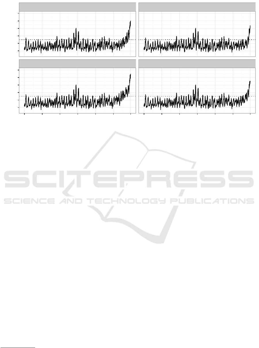
Bank Run A
Bank Run B
Bank Run C
Bank Run D
0.2
0.4
0.6
0.8
1.0
1.2
0.2
0.4
0.6
0.8
1.0
1.2
6770 7070 7370 7670 7970 8270 8560 6770 7070 7370 7670 7970 8270 8560
Time Interval
Reconstruction Error
Figure 4: The reconstruction error of the manipulated test sets estimated by the linear autoencoder for each time interval. We
simulated the bank runs at the final time intervals. The error curves are smoothed with a rolling average of ten time intervals
to make their trend more clearly visible. Moreover, the dotted line represents the anomaly threshold ε = 0.5.
holdout set was also randomly generated.
Before running the actual simulations, we deter-
mined how well the autoencoders were able to recon-
struct the original test set. Figure 3 shows the recon-
struction error estimated by the autoencoders for each
time interval. The error curves of the autoencoders
are quite similar and exhibit fluctuations. Moreover,
they display a short period of time, around time inter-
val 7670, were both autoencoders had difficulties re-
constructing the liquidity vectors. Closer inspection
revealed that these high errors were caused by a few
very large liquidity flows. No clear signs of stress
could be identified. Instead, we suspect that the large
errors were caused by random influences that are sub-
ject to the financial intermediation process.
We simulated the bank runs at the end of the test
set. Figure 4 shows the reconstruction error of the
manipulated test sets estimated by the linear autoen-
coder for each time interval
2
. The error curves were
smoothed by a rolling average of ten time intervals to
make their trend clearly visible. In addition, we ap-
plied an anomaly threshold of ε = 0.5.
The error curves clearly highlight the artificial
bank runs at the final time intervals. During these time
intervals, the reconstruction error increased rapidly as
the payment network started to change unexpectedly.
In particular, the stressed bank became more centrally
positioned having high outgoing liquidity flows to the
remaining banks in the payment network. We can see
2
The error curves of the sigmoid autoencoder are very
similar and omitted for brevity.
this when inspecting the reconstruction error of the
final liquidity matrices, see Figure 5. The high out-
going liquidity flows of the stressed bank could not
be accurately reconstructed and caused a high recon-
struction error during the bank runs.
6 CONCLUSIONS
We have introduced a method to detect system-level
anomalies in a RTGS system. This method involves
training an autoencoder to reconstruct a set of liquid-
ity vectors. Our experimental results show that liquid-
ity vectors contain distinctive features of a payment
network which an autoencoder is able to capture very
well. Furthermore, the reconstruction error made by
a well-trained autoencoder after compressing and re-
constructing the liquidity vectors reflects anomalous
changes in the liquidity flows between banks.
In the future, we plan to further improve our work
in several aspects. This includes: evaluating the pro-
posed method on larger payment networks that are
subject to real-world stress, explaining the most likely
cause of anomalies, and incorporating time dependen-
cies between liquidity vectors.
ACKNOWLEDGEMENTS
We would like to thank Ron Berndsen for his helpful
suggestions and feedback.
Anomaly Detection in Real-Time Gross Settlement Systems
439

(a) (b) (c)
Figure 5: The reconstruction error of the liquidity matrices at (a) t
8528
, (b) t
8529
, and (c) t
8530
of bank run C estimated by the
linear autoencoder. The intensity of each element indicates the error made by the autoencoder for the corresponding liquidity
flow. The fourth row from the top represents the outgoing liquidity flows of the stressed bank.
REFERENCES
Allen, F. and Gale, D. (2000). Financial Contagion. Journal
of Political Economy, 108:1–33.
Arciero, L., Heijmans, R., Heuver, R., Massarenti, M., Pi-
cillo, C., and Vacirca, F. (2016). How to Measure the
Unsecured Money Market? The Eurosystem’s Imple-
mentation and Validation using TARGET2 Data. In-
ternational Journal of Central Banking, March:247–
280.
Armantier, O. and Copeland, A. (2012). Assessing the
Quality of Furfine-based Algorithms. Federal Reserve
Bank of New York Staff Report, 575.
Berndsen, R. J., Le
´
on, C., and Renneboog, L. (2016). Fi-
nancial Stability in Networks of Financial Institutions
and Market Infrastructures. Journal of Financial Sta-
bility.
Bottou, L. (2004). Stochastic Learning. In Advanced lec-
tures on machine learning, pages 146–168. Springer.
Chandola, V., Banerjee, A., and Kumar, V. (2009).
Anomaly Detection: A Survey. ACM Comput. Surv.,
41(3):15:1–15:58.
Donoho, S. (2004). Early Detection of Insider Trading in
Option Markets. In Proceedings of the tenth ACM
SIGKDD international conference on Knowledge dis-
covery and data mining, pages 420–429. ACM.
Ferdousi, Z. and Maeda, A. (2006). Unsupervised Out-
lier Detection in Time Series Data. In 22nd Inter-
national Conference on Data Engineering Workshops
(ICDEW’06), pages 51–56. IEEE.
Furfine, C. (1999). The Microstructure of the Federal Funds
Market. Financial Markets, Institutions and Instru-
ments, 8:24–44.
Gai, P. and Kapadia, S. (2010). Contagion in financial net-
works. In Proceedings of the Royal Society of London
A: Mathematical, Physical and Engineering Sciences,
page rspa20090410. The Royal Society.
Ghosh, S. and Reilly, D. L. (1994). Credit card fraud de-
tection with a neural-network. In System Sciences,
1994. Proceedings of the Twenty-Seventh Hawaii In-
ternational Conference on, volume 3, pages 621–630.
IEEE.
Hawkins, S., He, H., Williams, G., and Baxter, R. (2002).
Outlier Detection Using Replicator Neural Networks.
In International Conference on Data Warehousing
and Knowledge Discovery, pages 170–180. Springer.
Heijmans, R. and Heuver, R. (2014). Is this Bank Ill? The
Diagnosis of Doctor TARGET2. Journal of Financial
Market Infrastructures, 2(3).
Kim, Y. and Sohn, S. Y. (2012). Stock fraud detection us-
ing peer group analysis. Expert Systems with Applica-
tions, 39(10):8986–8992.
Laine, T., K., K., and & Hellqvist, M. (2013). Simulations
Approaches to Risk, Efficiency, and Liquidity Usage in
Payment Systems. IGI Global.
Leinonen, H. and Soram
¨
aki, K. (2005). Optimising Liq-
uidity Usage and Settlement Speed in Payment Sys-
tems. In Leinonen, H., editor, Liquidity, risks and
speed in payment and settlement systems - a simula-
tion approach., Proceedings from the Bank of Fin-
land Payment and Settlement System Seminars 2005,
pages 115–148.
Le
´
on, C. and P
´
erez, J. (2014). Assessing financial mar-
ket infrastructures’ systemic importance with author-
ity and hub centrality. Journal of Financial Markt In-
frastructures.
Maes, S., Tuyls, K., Vanschoenwinkel, B., and Mander-
ick, B. (2002). Credit Card Fraud Detection Using
Bayesian and Neural Networks. In Proceedings of the
1st international naiso congress on neuro fuzzy tech-
nologies, pages 261–270.
Ng, A. (2011). Sparse autoencoder. CS294A Lecture notes,
72:1–19.
Quah, J. T. and Sriganesh, M. (2008). Real-time credit card
fraud detection using computational intelligence. Ex-
pert systems with applications, 35(4):1721–1732.
Rifai, S., Vincent, P., Muller, X., Glorot, X., and Bengio, Y.
(2011). Contractive Auto-Encoders: Explicit Invari-
ance During Feature Extraction. In Proceedings of
ICEIS 2017 - 19th International Conference on Enterprise Information Systems
440

the 28th international conference on machine learn-
ing (ICML-11), pages 833–840.
Rumelhart, D. E., Hinton, G. E., and Williams, R. J. (1985).
Learning Internal Representations by Error Propaga-
tion. Technical report, DTIC Document.
S
´
anchez, D., Vila, M., Cerda, L., and Serrano, J.-M. (2009).
Association rules applied to credit card fraud detec-
tion. Expert Systems with Applications, 36(2):3630–
3640.
Srivastava, A., Kundu, A., Sural, S., and Majumdar, A.
(2008). Credit Card Fraud Detection Using Hidden
Markov Model. IEEE Transactions on dependable
and secure computing, 5(1):37–48.
Vincent, P., Larochelle, H., Bengio, Y., and Manzagol, P.-A.
(2008). Extracting and Composing Robust Features
with Denoising Autoencoders. In Proceedings of the
25th international conference on Machine learning,
pages 1096–1103. ACM.
Werbos, P. J. (1982). Applications of Advances in Non-
linear Sensitivity Analysis. In System modeling and
optimization, pages 762–770. Springer.
Zaslavsky, V. and Strizhak, A. (2006). Credit Card Fraud
Detection Using Self-Organizing Maps. Information
and Security, 18:48.
Anomaly Detection in Real-Time Gross Settlement Systems
441