An Extrinsic Sensor Calibration Framework for Sensor-fusion based

Autonomous Vehicle Perception

Mokhtar Bouain

1,2

, Denis Berdjag

, Nizar Fakhfakh

and Rabie Ben Atitallah

Navya Company, Paris, France

LAMIH CNRS UMR 8201, University of Valenciennes, 59313 Valenciennes, France

Keywords:

Sensor Alignment, Sensor Calibration, Sensor Fusion, Intelligent Vehicles.

Abstract:

In this paper we deal with sensor alignment problems that appear when implementing sensor fusion-based au-

tonomous vehicle perception. We focus on extrinsic calibration of vision-based and line scan LIDAR sensors.

Based on state-of-art solutions, a consistent calibration toolchain is developed, with improvements (accuracy

and calibration duration). Additionally, sensor alignment/calibration impact on fusion-based perception is

investigated. Experimental results are provided for illustration, using real-world data.

1 INTRODUCTION

When dealing with robotic perception, single-sensor

architecture are range-limited. This limit depends

on many factors such as the technology of the de-

vice (resolution, range...), limited spatial and tempo-

ral coverage, measurement rates, noises... Indeed, any

cost-efﬁcient sensor will be optimized to deal with a

speciﬁc task. As a result, when dealing with percep-

tion tasks in a rich environment, such as object de-

tection and avoidance for robots or autonomous nav-

igation, using multiple sensors is a natural solution

(Baig et al., 2011). Multi-sensor perception requires

data fusion approaches to reconstruct world features

for the robot, based on synergistic and redundant mea-

surements. Data fusion is indeed widely used in many

ﬁelds of robotics such as perception (obstacle detec-

tions, environment mapping)(Wittmann et al., 2014)

and also in process control tasks. However combin-

ing homogeneous or heterogeneous measurements re-

mains a challenge to be tackled. Some of the key

issues are the diversity of the existing technologies

and the appearance of new sensor types. Other issues

are related to the application ﬁeld, for example, au-

tonomous vehicles will be driven in ”open” environ-

ments, and that implies stringent security constraints.

This research deals with the initial phase of any multi-

sensor acquisition, the alignment process. When fea-

tures are acquired for real world measurements, nor-

malization is required in order to reconstruct the IA

perceived word without bias, and take appropriate ac-

tions. We address speciﬁcally vision-based and LI-

DAR based sensor alignment, and derive a general

framework and the appropriate toolchain. Despite the

popularity topic, discussed in the next section, few

works address all the steps of the process. Then we

discuss the impacts of the calibration procedure on

fusion accuracy. This paper present three main con-

tributions:

• We develop further a speciﬁc framework pre-

sented in (Guo and Roumeliotis, 2013), and ex-

tend it from single to multi-line reference in or-

der to reduce the required number poses. In addi-

tion we address the problem of point-normal vec-

tor correspondences.

• we present a complete implementable toolchain,

to extract the co-features for both types of sen-

sors: line detections for cameras and segmenta-

tion process for LIDAR sensors in order to make

fully automated feature acquisition.

• we investigate the impact of the calibration accu-

racy on sensor fusion performance.

The remaining of this paper is organized as follows:

In section 2 we present a survey of existing methods

and point out the classiﬁcation of alignment methods.

In section 3 we describe the problem formulation and

we present the analytical least square solution to the

multi-line calibration approach. The co-feature ex-

traction is discussed in section 4. We detail the im-

pact of the calibration task of sensor-fusion accuracy

in section 5. Section 6 discusses the experimental

setup and tests using real data. The conclusion and

future work are discussed in section 7.

Bouain, M., Berdjag, D., Fakhfakh, N. and Atitallah, R.

An Extrinsic Sensor Calibration Framework for Sensor-fusion based Autonomous Vehicle Perception.

DOI: 10.5220/0006438105050512

In Proceedings of the 14th International Conference on Informatics in Control, Automation and Robotics (ICINCO 2017) - Volume 1, pages 505-512

ISBN: 978-989-758-263-9

505

2 RELATED WORK

Multi-sensor architectures are popular nowadays, and

research works on derived topics such as calibra-

tion are also plentiful, especially about visual, iner-

tial and LIDAR sensors. The authors of (Li et al.,

2013) classify extrinsic calibration methods of cam-

era and LIDAR sensors. According to this classiﬁca-

tion, there are three categories of camera/LIDAR cali-

bration: the ﬁrst method is based on auxiliary sensors;

using a third sensor which is Inertial Measurement

Unit (IMU), extrinsic calibration is carried out. It is

shown that the rigid transformation between the two

frames can be estimated using the IMU (Nez et al.,

2009). The second method is based on specially de-

signed calibration boards. The idea is to use a par-

ticular pattern to determine targets position in both

sensors frames, and subsequently express the target

coordinates in each frame in order to derive the rigid

transformations. In (Fremont et al., 2012), the cali-

bration uses circular targets for intelligent vehicle ap-

plications and dedicated to multi-layer LIDAR. This

method determines the relative pose in rotation and

translation of the sensors using sets of correspond-

ing circular features acquired for several target con-

ﬁgurations (Fremont et al., 2012). Similarly, (Park

et al., 2014) uses a polygonal planar board to perform

calibration of color camera and multi-layer Lidar for

robot navigation tasks. Concerning the third category,

it is about methods that use chessboard targets. This

kind of calibration is also pattern speciﬁc. The ad-

vantage of this method is determining the intrinsic

parameters simultaneously for cameras and extrinsic

calibration of the camera and the LIDAR (Li et al.,

2013). In addition to these three categories, we con-

sider another category which is the automatic extrin-

sic calibration. This kind of method is handled with-

out a designed calibration board or another sensor as

mentioned above. (John et al., 2015) proposes a cali-

bration approach does not need any particular shape to

be located. Their method consists to integrate the per-

ceived data from 3D LIDAR and stereo camera using

Particle Swarm Optimization algorithms (PSO), using

acquired objects from the outer world, without the aid

of any dedicated external pattern.

In addition, we can distinguish three main meth-

ods to solve the established closed form between the

correspondence features. The ﬁrst one solves the

closed form using linear methods such as the Singu-

lar Value Decomposition (SVD) and uses this solu-

tion as a ﬁrst guess to perform a nonlinear optimiza-

tion such as Gauss-Newton or Levenberg-Marquardt

algorithms. The second method is based on the idea

that the determination of the global minimum of a

given cost function needs to ﬁnd an initial guess lo-

cated in the basin of attraction. The authors of (Guo

and Roumeliotis, 2013) proposed an analytical least-

squares approach to carry out a generic calibration

process. The third method uses stochastic approaches

or search algorithms to associate the features between

two frames as the PSO algorithm, as it is shown in

(John et al., 2015). Based on the literature review,

we believe that the development of a generic solution

for sensor alignment is a viable solution. However in

the literature, little is said on the relationship between

sensor calibration and sensor fusion steps, apart from

automatic calibration approaches. We believe that

such contribution, for target-based solutions (shape or

pattern speciﬁc), is useful, especially if computation-

heavy algorithms (such as PSO) are avoided. In ad-

dition, few works address the tool-chain implementa-

tion on real vehicles. We believe that this topic is of

interest for practitioners.

3 PROBLEM FORMULATION

AND ANALYTICAL

LEAST-SQUARES SOLUTION

3.1 Problem Formulation and Basic

Concepts

The calibration process is an alignment procedure of

a given sensor frames. That is to say, ﬁnd the relation

between the coordinates of sensor frames to ensure

the transformation from a frame into another. Con-

cerning the extrinsic calibration of a LIDAR sensor

and camera, it is about estimation of the relative posi-

tion for a given point located in the real world frame,

in the LIDAR and camera frames. the objective is

to ﬁnd the unknown 6 Degrees Of Freedom (DOF)

transformation between the two sensor frames. In

other words, the goal is to ﬁnd the rigid transforma-

tion [

−→

], which allows us to determine the cor-

respondence of a given 3D LIDAR point represented

−→

= [x

]

located into the frame of the LI-

DAR sensor {L}, in the frame of the camera {C}. Let

−→

= [x

]

be the correspondence of

−→

(1)

Based on (Guo and Roumeliotis, 2013), we extend

the existing calibration solution to multi-line pattern

targets. We deﬁne the coordinate system for the sen-

sors as follows: the origin O

is the center of the

camera and the origin O

is the center of the LIDAR

sensor frame. Without loss of generality, the LIDAR

scanning plane is deﬁned as the plane z

= 0 (see

ICINCO 2017 - 14th International Conference on Informatics in Control, Automation and Robotics

506

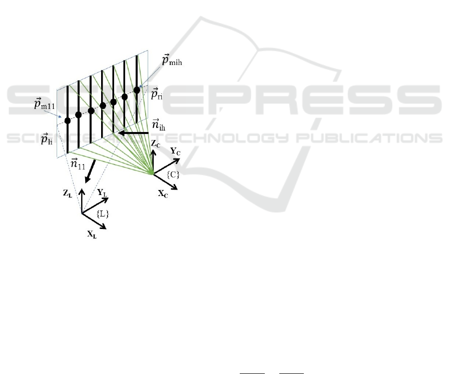
ﬁgure 1). Thus, a 3D LIDAR point represented as

−→

= [x

,0]

. We consider that the calibration

board contains d horizontal black lines lb

where h

is the number of line and i is the number of pose. It

is required to ﬁx these lines equidistant between each

other, i.e. if there are d lines, it is necessary that the

(d + 1) parts are equals. Assume that

−→

and

−→

are

respectively the left and right ending points of the pat-

tern. By dividing the distance between

−→

and

−→

by (d + 1), we get an estimation of the positions of

−→

mih

(Fig. 1). Otherwise, the normal vector

−→

perpendicular to the plane T

deﬁned by l

bih

and the

camera center. Since the correspondent of

−→

mih

the camera frame {C} belongs to the plane T

, then

−→

will correspond to

−→

mih

. Therefore, we obtain

the following geometric constraints:

−→

cih

−→

(

−→

mih

−→

) = 0 (2)

where

−→

cih

is the correspondent of the LIDAR point

−→

mih

in the camera frame.

Figure 1: Notations and geometric constraints.

In real-world situations (2) is never satisﬁed due to

the measurement noise and it will usually be slightly

different from zero. The difference is the error e

. All

the residuals for n measurements can be represented

−→

e = (

−→

(

−→

m11

−→

(

−→

m12

−→

)

,...

−→

(

−→

mnd

−→

))

(3)

To estimate the transformation parameters [

−→

]

with accurately and minimize the residuals from (3),

we deﬁne the cost function J and we aim to minimize

the sum of squared errors :

J = argmin

∑

i=1

∑

h=1

)

(4)

J = argmin

∑

i=1

∑

h=1

(

−→

(

−→

mih

−→

))

s.t.

= I, det(

) = 1

(5)

The two above conditions represent the rotational ma-

trix constraints.

We now have a correspondence between a 3D point

in LIDAR frame and the plane deﬁned by O

and

the black lines in the camera frame. First, accord-

ing to (2) and for h = 1...d,

and

−→

are the

unknowns. Second, let

−→

and

−→

be the three

columns of

. Since the LIDAR scanning plane is

deﬁned as the plane z

= 0 then we do not have an

explicit dependence on

−→

and hence we can rewrite

−→

(× is the cross product).

To summarize, we get nine unknowns grouped in

−→

and

−→

and three constraints since

an orthonormal matrix.

3.2 Closed-form Solution

3.2.1 Redeﬁning the Optimization Problem

The objective is to solve the equation (5) to ﬁnd the

parameters of calibration. The ﬁrst step consists to

reduce the number of variables and constraints in (5).

Since the translation,

−→

is not involved in the con-

straints, it can be eliminated from the optimization

problem.

Lemma 1: By reducing the number of variables in (5)

the cost function is deﬁned as follows:

J =

∑

i=1

∑

h=1

−→

mih

− (

∑

j=1

∑

l=1

−→

ih jl

−→

m jl

)

s.t.

= I, det(

) = 1

(6)

where:

−→

ih jl

−→



∑

j=1

∑

l=1

−→



−1

−→

= −



∑

i=1

∑

h=1

−→



−1



∑

i=1

∑

h=1

−→

mih



(7)

Proof: By applying the ﬁrst order necessary condi-

tion for optimality to the cost function, we obtain:

∂J

∂

−→

∂

−→



∑

i=1

∑

h=1

(

−→

(

−→

mih

−→

))



∑

i=1

∑

h=1

−→

mih

−→

= 0

An Extrinsic Sensor Calibration Framework for Sensor-fusion based Autonomous Vehicle Perception

507

−→

= −F

−1



∑

i=1

∑

h=1

−→

mih



(8)

Where :

F =



∑

i=1

∑

h=1

−→



J =

∑

i=1

∑

h=1

−→

mih

−

−→

−1

(

∑

j=1

∑

l =1

−→

m jl

)

∑

i=1

∑

h=1

−→

mih

− (

∑

j=1

∑

l =1

−→

−1

−→

m jl

)

And hence, the cost function is expressed only by

the rotation matrix and its constraints:

J =

∑

i=1

∑

h=1

−→

mih

− (

∑

j=1

∑

l=1

−→

ih jl

−→

m jl

)

3.2.2 Simplifying Optimization Problem using

Quaternion Unit

To simplify the problem and reduce further the num-

ber of unknowns, the quaternion unit q is employed

to represent the rotation matrix

. The conversion

from vectors to quaternions and all the quaternion

parameterization are presented in the appendix.

Lemma 2: By using the quaternion units, (6) can be

written as follows:

J =

∑

i=1

∑

h=1

s.t.

= 1

(9)

where :

= L( ¯n

)

R ( ¯p

mih

) −

∑

j=1

∑

l=1

L( ¯w

ih jl

)

R ( ¯p

m jl

)

where L (.) and R (.) are left and right quaternion

multiplication matrices (see appendix for details).

Proof: Based on quaternion calculus properties, con-

version of 3D vectors into quaternions and quaternion

multiplication, we can rewrite the cost function as fol-

lows:

J =

∑

i=1

∑

h=1

−

(q ⊗ ¯p

mih

⊗ q

−1

) −

∑

j=1

∑

l =1

−

ih jl

(q ⊗ ¯p

m jl

⊗ q

−1

)

∑

i=1

∑

h=1

−

(L(q) ¯p

mih

⊗ q

−1

) −

∑

j=1

∑

l =1

¯w

ih jl

(L(q) ¯p

m jl

⊗ q

−1

)

Since (L (q) ¯p

mih

) ⊗q

−1

= R (q

−1

)(L(q) ¯p

mih

)

and (L (q) ¯p

m jl

) ⊗q

−1

= R (q

−1

)(L(q) ¯p

m jl

)

Then :

J =

∑

i=1

∑

h=1

−

R (q

−1

)L(q) ¯p

mih

−

∑

j=1

∑

l =1

−

ih jl

R (q

−1

)L(q) ¯p

m jl

Since L (q) ¯p

mih

= R ( ¯p

mih

and L (q) ¯p

m jl

= R ( ¯p

m jl

Then the the cost function is reformulated as the following :

J =

∑

i=1

∑

h=1

L( ¯n

)

R ( ¯p

mih

)q −

∑

j=1

∑

l =1

L( ¯w

ih jl

)

R ( ¯p

m jl

∑

i=1

∑

h=1



L( ¯n

)

R ( ¯p

mih

) −

∑

j=1

∑

l =1

L( ¯w

ih jl

)

R ( ¯p

m jl

)



3.2.3 Lagrange Multiplier Method

In order to solve the equation form Lemma 2, we

show now how to formulate the problem as a set of

polynomial equations. To solve the cost function J

we use the Lagrange multiplier method. According

to the Lagrange method, the Lagrangian function is

deﬁned as follows:

L(q,λ) = J(q) + λ(

q q − 1) (10)

Where λ is the Lagrange multiplier.

Hence, using the method of Lagrange multiplier, we

obtain the following equations:











∑

i=1

∑

h=1

+ S

q + λq = 0

q q − 1 = 0

(11)

3.3 The Problem of Point-normal

Vector Correspondences

The use of point-normal vector correspondences is

strongly impacted by the quality of LIDAR endpoint

detection. Sometimes, the LIDAR endpoint will not

exactly locate on the border of the calibration tar-

get. In order to overcome this problem, the authors

of (Lipu and Zhidong, 2014) have proved that plac-

ing the calibration target nearby the LIDAR sensor

provides a high quality line-point correspondence and

sufﬁcient constraints to estimate the rigid transforma-

tion. In addition, we present a method to improve

the accuracy of the endpoint estimation using virtual

points. The positions of the virtual points are deter-

mined by the average distance between the points of

LIDAR for each pose. So, if

−→

and

−→

are the end-

ing points of calibration board (left and right side), the

average Euclidean distance is calculated as follows :

lri

dist(

−→

)

(12)

where n is the number of scanned point located on the

pattern. So, the positions of the left and right virtual

points are :

−→

V li

−→

−

lri

−→

V ri

−→

lri

−→

where

−→

u =

−→

−

−→

ICINCO 2017 - 14th International Conference on Informatics in Control, Automation and Robotics

508

4 PREPROCESSING AND

FEATURE EXTRACTION

4.1 Extraction of 3D LIDAR Points

To extract the projected points of the source sensor

on the calibration board, the automatic extraction ap-

proach by differentiation of the measurements and

background data in static environments is often used.

However, in this work, this task is carried out by using

a segmentation process. Each segment (cluster) is de-

ﬁned as a set of points and is composed ofa minimum

number of points distant according to a threshold dis-

tance denoted T hr. Therefore, if dist(

−→

i+1

) <

T hr then a segment is deﬁned with C

as its centroid.

Where,

−→

is the impact point of the LIDAR sensor,

dist(

−→

i+1

) is the Euclidean distance between two

adjacent points and T hr is the required threshold. The

coordinate of each centroid C

is calculated as follows:

(

∑

) where n is the number of points. We can

add another parameter to ﬁx the minimum number of

points that compose a segment. Figure 2 shows the

projected impact points on the target and its environ-

ment.

Figure 2: Projected impact points (environment).

4.2 Extraction of Lines using Hough

Transform

Hough transform is considered to be an efﬁcient

method to locate lines. The idea is to transform every

point in x − y space (Cartesian frame) into parameter

space (Polar frame). This method deﬁnes two param-

eters spaces which are r the length of a normal from

the origin of this line and θ is the orientation of r with

respect to the x − axis. Hence the line equation for

each line is r = x cos(θ) + ysin(θ). After the trans-

formation of all points into the parameter space, local

peaks in the parameter space associated to line candi-

dates in x − y space can be extracted. Otherwise, the

line detection chain consists of a set of instructions.

Before using the Hough transform it is necessary to

apply a spatial ﬁlter to the image in order to reduce

the noise. Among existing spatial ﬁlters, we use the

Gaussian smoothing which is a 2-D ﬁlter of images

that is used to remove/reduce the details and noises

and also to blur images. Mathematically, applying the

Gaussian smoothing ﬁlter it is the same as convolv-

ing the image with a Gaussian kernel. The main idea

is that the new pixels of the image are created by a

weighted average of the pixels close to it (gives more

weight to the central pixels and less weights to the

neighbors). After the removal of details and noises,

the edges of the image will be extracted using an edge

detector algorithm. It allows us to ﬁnd the boundary

of objects and hence extract useful structural infor-

mation in order to reduce the amount of data to be

processed. Mainly there are two commonly used ap-

proaches for edge detection which are Canny and So-

bel edge detector (the difference of these approaches

is the kernel in that they are using). In this work, we

use the Canny edge detector. It is based on ﬁnding

the intensity gradient of the image, and according to

ﬁxed thresholds, a pixel will be accepted as an edge

or rejected. At this stage, the Hough transform is ap-

plied. Note that there are additional steps are taken

to perform the extraction of black lines, such as limit-

ing the regions of interest to reduce the computational

burden. Also, it is necessary to ﬁlter false detections

and keep only the inlier lines. To do this, we use a

priori knowledge because we know that we need only

the vertical lines and concerning the horizontal lines

(or close to be), they are eliminated according to their

slopes. In addition, we use another criterion which is

the color of lines that are looking which is the black

therefore we keep the lines that have the black color.

5 SENSOR CALIBRATION

ACCURACY IMPACT ON

MULTI-SENSOR DATA FUSION

In order to fuse the data between sensors, it is neces-

sary to estimate or model the errors that are involved

in the data processing level. These errors will be used

to represent the uncertainties of sensors and to weigh

the measurements during the fusion process. Sensor

uncertainties are caused by many types of errors. We

distinguish two main types: the random errors which

An Extrinsic Sensor Calibration Framework for Sensor-fusion based Autonomous Vehicle Perception

509

are the noise measurements and the calibration errors

which are caused by the alignment process. There-

fore a multi-sensor data fusion should take into ac-

count these errors to improve its quality. The authors

of (Baig et al., 2011) use the Bayesian Fusion tech-

nique to fuse the positions acquired by two sensors in

the context of environment perception of autonomous

vehicles.

The sensors are employed to detect the positions

of obstacles. Position uncertainty is represented using

2D Gaussian distribution for both objects. Therefore,

if X is the true position of the detected object, by using

the Bayesian fusion, the probability of fused position

]

by the two sensors is given as:

rob

(P|X) =

−(P−X)

−1

(P−X)

2π

|R|

(13)

where P is the fused position and R is the covariance

matrix are given as :

P =

+ P

1/R

+ 1/R

and 1/R = 1/R

+ 1/R

where P

and R

are the position and covariance ma-

trix of sensor 1 and P

and R

are that of sensor 2.

We acquire positions of the detected obstacles by both

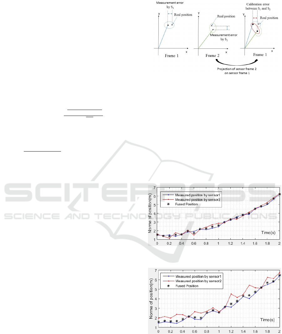
sensors. Figure 3 shows the modeled error positions

of one detected obstacle by two sensors. The cross

represents the real positions which are unknown, the

two black dots represent the measurements of posi-

tions, the circles (red and green) are the position un-

certainties. The red circle is the calibration uncer-

tainty which is generated by the calibration process

which we are aiming to minimize. We test the im-

pact of the calibration process on a multi-sensor data

fusion based on Bayesian approach by varying the

covariance matrices of sensors. The noise measure-

ments will be Gaussian noises with zero mean and the

standard deviation is 120 mm for both of sensors. The

dynamic model of position is modeled by a rectilinear

motion. Note that R

= R

i.e. the covariance matrix

of sensor 1 contains only the error of measurements.

In contrast, R

= R

+ R

i.e. the covariance of sen-

sor 2 contains both measurement and calibration er-

rors (because the measurements of sensor 2 will be

projected on the frame of sensor 1). To summarize,

in the ﬁrst simulation, the calibration error of sensor

2 will be small while in the second simulation we will

increase its calibration error.

Figures 4 and 5 show the obtained results: the norm

of position (meter) for each sensor with two conﬁgu-

rations of calibration errors over time. It is clear that

in the ﬁrst simulation (Figure 4: when the sensor 2

has a small value of calibration error), the fused posi-

tion is located between the two provided positions by

Figure 3: Measurement and calibration errors.

the sensors. In contrast, in the second simulation and

when the calibration error rises, the fused position fol-

lows the position provided by sensor 1, because it has

the smallest error (see ﬁgure 5). According to these

experiments, it is clear that the outcome is a combina-

tion of the two measurements weighted by their noise

covariance’s matrices. Therefore, if the calibration

error grows then the projection of the measurement

of sensor 2 will be distorted, so the combined result

follows uniquely the measurement of the ﬁrst sensor

(Figure 5). This makes the use of sensor 2 obsolete

and demonstrates the advantages of the multi-sensor

data fusion architecture.

Figure 4: Fusion of two positions weighted with similar co-

variance matrices.

Figure 5: Fusion of two positions with the increase in the

calibration error of sensor 2.

In practice, it is difﬁcult to obtain or evaluate the

ground truth of the real extrinsic parameters between

the camera and LIDAR sensors. There are some

works deﬁne theirs own criteria. For our work we

propose the sum of squared residuals as an indicator

ICINCO 2017 - 14th International Conference on Informatics in Control, Automation and Robotics

510

of calibration. As long as this criterion tends to 0 we

will get a good performance of calibration process.

6 EXPERIMENTS

In order to validate the multi-line approach, we con-

ducted a series of experiments in the real environ-

ment. We use line-scan LIDAR with an angular res-

olution 0.25 degree and a color camera with 640x480

resolution. The camera is modeled using a pinhole

model. The number of point-normal vector corre-

spondences is ﬁxed to three. We use a white calibra-

tion board with three black lines (d = 3). Note that a

chessboard pattern is also usable.

6.1 Extraction of Lines from

Calibration Board

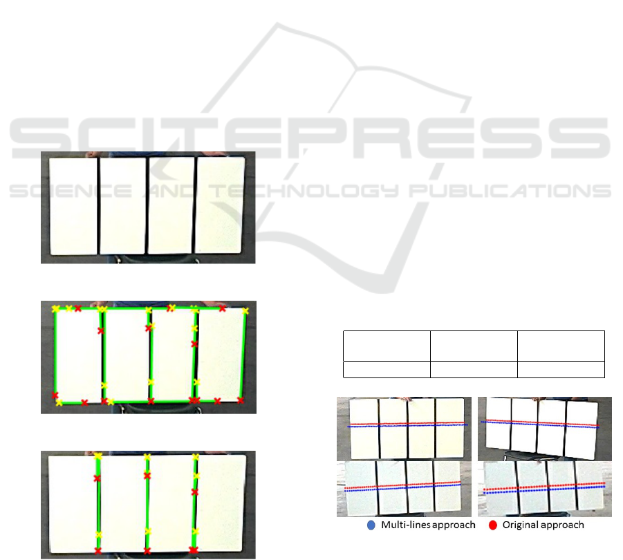
Figure 6 shows the calibration board with three black

lines. We use an image processing algorithm based

on Hough Transform to extract the lines. Figure 7

shows a partial result that contain some false detec-

tions other than the black lines (Figure 8). To remove

the false detections, we perform ﬁltering and keep just

the three black lines (see section 6.1). Therefore, from

Figure 6: The used pattern for calibration (3 black lines).

Figure 7: Line detections using Hough Transform.

Figure 8: Keeping the black lines of the calibration board.

each line we need two points to determine the normal

vectors.

6.2 Results of Camera LIDAR

Calibration

For the original (existing) approach, we collected 21

point-normal vector correspondences to estimate cali-

bration parameters and used only 7 poses for the mod-

iﬁed approach. The calibration board was moved to

a 3m to 9m distance range. To compare the results,

the average between the pixel coordinates of LIDAR

points for different poses is calculated. Table 1 shows

the results. The shown results correspond to the av-

erage absolute distance for u axis, v axis and the av-

erage Euclidean distance between the correspond pix-

els. According to these results, the two implementa-

tions are very close. Therefore, the result of the multi-

lines approach is well performed as original approach

with beneﬁts reducing the required number of poses.

Otherwise, in order to suppress or at least reduce

the effect of noise during measurements, it is reason-

able to use multiple observations of the calibration

pattern from different views to obtain the required

6 DOF. Also, it is required to rotate the calibration

board to allow normal vector

−→

to span all three di-

rections.

Figure (9) shows the projection results for the

two approaches for different orientations. Visually, it

is clear that there is a small difference between the

projected points for both of methods. It is due to

the different noises measurements and the polynomial

equation solver behavior. In fact, equation (11) has

a ﬂoating-point coefﬁcients and it is not possible to

get the same solution because the measurements and

noises will be varying from one data set to another.

Table 1: The average difference between the two ap-

proaches.

Mean ”u”

dist. (pixel)

Mean ”v”

dist. (pixel)

Mean

dist. (pixel)

2.399 3.6816 3.3927

Figure 9: Projection of the LIDAR points into the image

plane.

An Extrinsic Sensor Calibration Framework for Sensor-fusion based Autonomous Vehicle Perception

511

7 CONCLUSIONS

In this paper, we address the problem of the frame

alignment between a camera and a 2-D LIDAR sensor

through the extended generic framework. The origi-

nal problem formulation implies using a given num-

ber of calibration poses is improved to use less poses.

When compared to other approaches which accuracy

depends on a precise initial guess, the proposed solu-

tion is formal and gives an optimal result for a given

calibration poses batch. We proved that with such

method, the number of observations can be reduced

for an accurate result. In addition, a tool-chain is de-

rived to extract sensor-acquired co-features. Real ex-

periments conﬁrmed that the presented development

is beneﬁcial for our application. Future works will

deal with a native integration of the alignment pro-

cess in the fusion algorithm, with an expected real-

time sensor realignment module to deal with inaccu-

rate initial calibration.

ACKNOWLEDGEMENTS

The authors would like to think Navya company

who provided the data set and the platform of ex-

periments. This research is ﬁnancially supported by

Navya company and ANRT CIFRE program grant

from the French Government.

REFERENCES

Baig, Q., O., A., Trung-Dung, V., and Thierry, F. (2011).

Fusion Between Laser and Stereo Vision Data For

Moving Objects Tracking In Intersection Like Sce-

nario. In IV’2011 - IEEE Intelligent Vehicles Sympo-

sium, pages 362–367, Baden-Baden, Germany.

Fremont, V., Florez, S. A. R., and Bonnifait, P. (2012). Cir-

cular targets for 3d alignment of video and lidar sen-

sors. Advanced Robotics, 26:2087–2113.

Guo, C. X. and Roumeliotis, S. I. (2013). An analytical

least-squares solution to the line scan lidar-camera ex-

trinsic calibration problem. In Robotics and Automa-

tion (ICRA), 2013 IEEE International Conference on,

pages 2943–2948. IEEE.

John, V., Long, Q., Liu, Z., and Mita, S. (2015). Auto-

matic calibration and registration of lidar and stereo

camera without calibration objects. In 2015 IEEE In-

ternational Conference on Vehicular Electronics and

Safety (ICVES), pages 231–237.

Li, Y., Ruichek, Y., and Cappelle, C. (2013). Optimal ex-

trinsic calibration between a stereoscopic system and

a lidar. IEEE Transactions on Instrumentation and

Measurement, 62(8):2258–2269.

Lipu, Z. and Zhidong, D. (2014). A new algorithm for

the establishing data association between a camera

and a 2-d lidar. Tsinghua Science and Technology,

19(3):314–322.

Nez, P., Drews, P., Rocha, J. R. P., and Dias, J. (2009).

Data fusion calibration for a 3d laser range ﬁnder and

a camera using inertial data. In ECMR, pages 31–36.

Park, Y., Yun, S., Won, C. S., Cho, K., Um, K., and Sim, S.

(2014). Calibration between color camera and 3d lidar

instruments with a polygonal planar board. Sensors,

14(3):5333–5353.

Trawny, N. and Roumeliotis, S. I. (2005). Indirect kalman

ﬁlter for 3d attitude estimation. University of Min-

nesota, Dept. of Comp. Sci. & Eng., Tech. Rep, 2:2005.

Wittmann, D., F., C., and M., L. (2014). Improving lidar

data evaluation for object detection and tracking using

a priori knowledge and sensorfusion. In Informatics

in Control, Automation and Robotics (ICINCO), 2014

11th International Conference on, volume 1, pages

794–801. IEEE.

APPENDIX

- The quaternion is generally deﬁned as

¯q = q

+ q

i + q

j + q

k (14)

where i, j, and k are hyper-imaginary numbers and the

quantity q

is the real or scalar part of the quaternion.

- To convert a 3D vector

−→

p to quaternion form we use

¯p = [

−→

p 0]

(15)

-The product

−→

= R

−→

where

−→

are vectors,

R is the rotation matrix and q its quaternion equiva-

lent, can be written as follow

¯p

= q ⊗ ¯p

⊗ q

−1

(16)

where ⊗ presents quaternion multiplication, q

−1

the quaternion inverse deﬁned as q

−1

= [−q

− q

−

]

-For any quaternions q

and q

, the product, q

⊗ q

is deﬁned as

⊗ q

, L(q

= R (q

(17)

Where:

L(q) =







−q







R (q) =







−q







Also we have following properties

L(q

)R (q

) = R (q

)L(q

)

L(q

)

= q

R (q

)

L(q

−1

) = L(q)

R (q

−1

) = R (q)

For more details, the interested reader is referred to

(Trawny and Roumeliotis, 2005).

ICINCO 2017 - 14th International Conference on Informatics in Control, Automation and Robotics

512