
A Methodology to Compare Different Co-simulation Interfaces:
A Thermal Engineering Case Study
Georg Engel, Ajay S. Chakkaravarthy and Gerald Schweiger
AEE - Institute for Sustainable Technologies, Feldgasse 19, Gleisdorf, Austria
Keywords:
Co-simulation, FMI, BCVTB, Trnsys, Simulink, Compact Thermal Energy Storage.
Abstract:
A method is presented to compare different co-simulation interfaces and applied to a case study of thermal
engineering. Different interfaces providing loose and strong coupling based on the Functional Mockup In-
terface (FMI), the Building Controls Virtual Test Bed (BCVTB) and a Component Object Model (COM)
are compared with respect to user-friendliness and flexibility, computational costs and accuracy. The case
study considered includes a compact thermal energy storage modelled in Trnsys and a heat sink modelled in
Simulink. The implemented strong coupling scheme is a factor of 10 more accurate while a factor of almost
100 computationally more demanding than the loose coupling one.
1 INTRODUCTION
1.1 Motivation and Background
The need for co-simulation is a pragmatic one:
Complex models are usually decomposed into sub-
systems, where different tools and methods are used
by different teams to implement these sub-systems.
This can be seen in many application areas such as the
design of energy-systems, automotive industry or any
interdisciplinary field. The need for co-simulation in
the field of energy systems arises from the goal of the
energy transition: (i) existing systems must become
more efficient and (ii) as fluctuating energy sources
such as wind and solar energy expand, other parts
of the energy systems must become more flexible to
match the available energy from renewable resources
with the demand in terms of location, time and quan-
tity. There are a number of options for increasing
energy system flexibility, including combining differ-
ent energy domains, increasing supply and demand
flexibility or integrating energy storage technologies
(Lund et al., 2015; Schweiger et al., 2017). In the
automotive sector, the transition to e-mobility poses a
variety of challenges. Considering the lack of waste
heat and the narrow temperature window required by
the battery, a smart thermal management of vehicles
including thermal storage becomes increasingly im-
portant (Bandhauer, 2011; Engel et al., 2017). This
leads to new requirements for simulation approaches
and tools. To increase the efficiency of existing sys-
tems, detailed models of all sub-systems that capture
all important dynamics are required.
In order to study different system solutions that
increase the system flexibility, completely new chal-
lenges need to be overcome such as (i) the coupling
of different domains and (ii) increased sub-system
dynamics as a result of this coupling; this leads to
new challenges for some domains. The simulation
of specific solutions provides the necessary insights
and information to support the transformation pro-
cess towards sustainable energy systems. There are
already tools for all domains and aspects of district-
scale energy systems, but no single tool can cover
all domains and aspects in order to simulate the en-
tire system (Allegrini et al., 2015). Co-simulation
approaches allow for the combination and reuse of
existing tools and methods that are robust and well-
suited for their particular domain. Models of different
sub-systems require different modelling approaches
and hugely differing step sizes or even solver algo-
rithms. Further advantages of co-simulation are (i)
it facilitates cross-discipline and cross-company col-
laborations, (ii) the possibility to protect model intel-
lectual property rights of sub-systems, (iii) robust co-
simulation frameworks can significantly shorten the
innovation cycle (robust prototyping) of novel system
and control concepts. F.i. different control algorithms
can be tested virtually at a system model without fur-
ther modification. A main drawback of co-simulating
is that numerical stability problems may arise (Tr-
cka et al., 2009), code optimizations within a partic-
410
Engel, G., Chakkaravarthy, A. and Schweiger, G.
A Methodology to Compare Different Co-simulation Interfaces: A Thermal Engineering Case Study.
DOI: 10.5220/0006480204100415
In Proceedings of the 7th International Conference on Simulation and Modeling Methodologies, Technologies and Applications (SIMULTECH 2017), pages 410-415
ISBN: 978-989-758-265-3
Copyright © 2017 by SCITEPRESS – Science and Technology Publications, Lda. All rights reserved
ular tool may be lost (Wetter et al., 2015) and some
co-simulation frameworks have inconvenient appli-
cation programming interfaces so that such methods
are inappropriate for engineering applications. An
overview of co-simulation approaches and tools, re-
search challenges, and research opportunities are pre-
sented in (Gomes et al., 2017; Trcka, 2008; Atam,
2017; Mathias et al., 2015). In (Gomes et al., 2017),
co-simulation approaches are divided into three cat-
egories: discrete event, continuous time and hybrid
co-simulations. The standard is stated to be FMI for
continuous time co-simulations and High Level Ar-
chitecture for discrete event ones, while no standard is
yet available for hybrid co-simulation. (Arnold et al.,
2013) present an error estimation for co-simulations
based on classical Richardson extrapolation, and a
modified algorithm for a reliable communication step
size control based on an extension of the step size con-
trol of classical time integration. They conclude that
the numerical efficiency of co-simulation algorithms
may be improved by higher-order approximations of
subsystem inputs.
The present work discusses a comparison of dif-
ferent free-of-charge co-simulation interfaces for con-
tinuous time between Trnsys and Simulink for a case
study in thermal engineering. The main contributions
of this paper are:
• A methodology to compare different co-
simulation interfaces is proposed.
• A strong coupling co-simulation interface be-
tween Trnsys and Simulink based on Type155 is
discussed.
• The methodology and the new strong coupling in-
terface are discussed for a case study typical for
thermal engineering.
• The results serve for a qualitative evaluation and
recommendation.
1.2 Tools and Interfaces
FMI (Blochwitz et al., 2009) is a tool independent
standard that has been developed in the ITEA2 Euro-
pean Advancement project MODELISAR. FMI sup-
ports both model exchange and co-simulation of dy-
namic models using a combination of xml-files and
compiled C-code. FMI is currently supported by 95
tools and is used by various industries and universi-
ties.
Trnsys is a simulation environment for the dy-
namic simulation of thermal systems, originally writ-
ten in the Fortran programming language (Klein et al.,
1976). Trnsys Type 155 implements a direct link
with Matlab. The connection uses the Matlab en-
gine, which is launched as a separate process. The
Fortran routine communicates with the Matlab engine
through a COM interface. Type 155 can be used in
different calling modes (standard component called in
each iteration or real-time controller called only after
convergence).
BCVTB is a software environment developed
at Lawrence Berkeley National Laboratory (Wetter,
2011). It allows connecting different simulation tools
to exchange data during the time integration. BCVTB
is based on Ptolemy II, an open-source software
framework supporting experimentation with actor-
oriented design. BCVTB has interfaces to Energy-
Plus, Dymola, Functionl Mock-up Units (FMU), Mat-
lab and Simulink, Radiance, ESP-r, Trnsys and BAC-
net.
The coupling between the different tools can be
done by either loose (also known as quasi-dynamic or
ping-pong coupling) or strong coupling (also known
as fully-dynamic or onion coupling) (Trcka, 2008). In
loose coupling, the data exchange between simulators
is realized only at certain points in time. There is no
iteration between the coupled simulators. Strong cou-
pling methods iterate the values needed from other
partial systems in every time step. Generally, the
strong coupling shows higher accuracy and higher sta-
bility at the costs of a higher computational time con-
sumption (Hafner et al., 2013).
2 METHOD
2.1 System Design
Interface for
Co-Simulation
Compact thermal
energy storage (T
s
)
Heat exchange via
heat transfer fluid
Heat sink - one
thermal node (T
b
)
Trnsys
model
Simulink
model
T
s,out
T
s,in
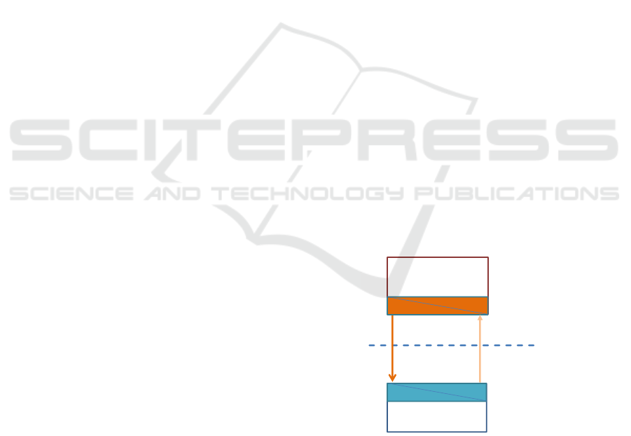
Figure 1: The physical system to be discussed as case study
for different co-simulation interfaces. A compact thermal
energy storage is connected to a heat sink with one thermal
node via a heat transfer fluid. The storage is modelled in
Trnsys, while the heat sink is modelled in Simulink.
In order to present the method and to compare
different co-simulation interfaces, we introduce a
toy example where a sorption-based compact ther-
mal energy storage is coupled thermally to a sim-
A Methodology to Compare Different Co-simulation Interfaces: A Thermal Engineering Case Study
411
ple heat sink. The corresponding system design is
shown in Figure 1. We discuss continuous time co-
simulation only, which is why discrete events like
control switches are avoided. Therefore, only dis-
charging of the storage is considered, where the sorp-
tion process releases heat, increasing the temperature
of the storage. The heat is extracted via a heat tranfer
fluid to the heat sink, which is represented by a simple
body with one thermal node.
2.2 Comparison with a Reference
Simulation
The different interfaces are compared with respect to
user-friendliness and flexibility, accuracy and compu-
tational costs. The user-friendliness and the flexibility
is judged only on a qualitative basis.
The model is implemented also entirely in Trnsys,
referred to as “reference simulation”, employed with
improved solver parameters (time step of 0.1 sec and
solver tolerance of 10
−7
) to ensure high accuracy re-
sults. These serve for a discussion of the accuracy of
the various co-simulations. The variables communi-
cated via the co-simulation interface (inlet and out-
let temperature of the heat transfer fluid) as well as
the temperatures of the heat storage and the body are
compared to the corresponding time-series results ob-
tained in the reference simulation. The maximum de-
viation is considered as measure for the accuracy.
To discuss the computational costs, a simple
batch-script is used to measure the overall simulation
time. This includes overhead like starting Matlab etc.,
but this is in most cases the relevant timing for the
user. Replica simulations serve to estimate the confi-
dence interval.
3 MODEL
3.1 Heat Storage - Trnsys Model
The compact thermal energy storage is modelled in
Trnsys as depicted in Figure 2. A more detailed de-
scription of the model is found in (Engel et al., 2017),
results were presented also in (Engel et al., 2016).
The following system of ordinary differential
equations is used to model the inner states of the sorp-
tion store, i.e. store temperature T
s
(energy balance,
Equation (1)) and water load of the sorption material
x
s
(mass balance, Equation (2)) (Engel et al., 2017):
C
tot
dT
s
dt
=
˙
Q
HX
+
˙
Q
vap,in
+
˙
Q
ads
+
˙
Q
amb
(1)
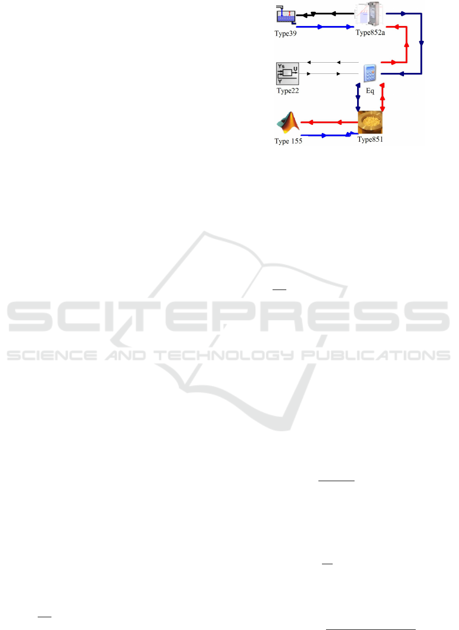
Figure 2: Model of the thermal energy storage in Trnsys
shown examplarily for the interface based on the Type155.
Type851 represents the sorption reactor, Type 852a the
evaporator/condenser, Type39 a water reservoir and Type22
and the equation block serve to calculate the vapour pres-
sure between the reactor and the evaporator/condenser. For
the reference simulation, Type155 is replaced by a Type rep-
resenting a counter-flow heat exchanger with one thermal
node at the secondary side. For the FMU-export, Type155
is replaced by Type6139a and Type6139b for input and out-
put, respectively.
dx
s
dt
= k
LDF
x
s,equ
(p
vap
, T
s
) − x
s
, (2)
where t denotes time, C
tot
the total (sensible) heat ca-
pacity of the sorption store, and k
LDF
the linear driv-
ing force parameter for adsorption and desorption, re-
spectively (Glueckauf, 1955). x
s,equ
= x
s,equ
(p
vap
, T
s
)
is the equilibrium water load of the sorption material,
calculated for the current store temperature T
s
and va-
por pressure p
vap
, e.g. by the Dubinin approach (Du-
binin, 1967). The different terms on the right hand
side of Equation 1 represent the heat flows for the
sorption store. The heat flow via the heat exchanger
(subscript “HX”), using the one-node approximation,
i.e., constant temperature T
s
= const., is calculated by
˙
Q
HX
= UA
HX
∆T
log
(T
s
, T
s,in
) (3)
=
"
1 − e
−UA
s,HX
˙m
HTF
c
p,HTF
#
˙m
HTF
c
p,HTF
(T
s,in
− T
s
)
˙m
HTF
denotes the mass flow of the heat transfer fluid,
and c
p,HTF
its heat capacity. T
s,in
(and T
s,out
) are the
inlet (and outlet) temperatures of the sorption reactor
fixed bed heat exchanger. The vapour mass flow is
given by ˙m
vap
= m
0
dx
s
dt
.
The evaporation/condensation kinetics is mod-
elled linear in the driving pressure difference, result-
ing in a vapor mass flow according to
˙m
vap
(T
2
) =
(βA)
p
vap
− p
sat
(T
2
)
R
vap
T
2
, (4)
SIMULTECH 2017 - 7th International Conference on Simulation and Modeling Methodologies, Technologies and Applications
412

where R
vap
denotes the gas constant of water vapor,
βA is the mass transfer coefficient characterizing the
linearized kinetics, and p
sat
(T
2
) is the saturation va-
por pressure for a given temperature T
2
. The vapour
mass flow between the sorption store and the evap-
orator/condenser is finally determined using an addi-
tional iterative solver (Type22).
3.2 Heat Sink - Simulink Model
As heat sink, a simple body with one thermal node
and a counter-flow heat exchanger is modelled by
dT
b
dt
=
˙m
HTF
c
p,HTF
m
b
c
p,b
1 − e
−UA
HX
˙m
HTF
c
p,HTF
(T
s,out
− T
b
)
(5)
T
s,in
= T
s,out
−
1 − e
−UA
HX
˙m
HTF
c
p,HTF
(T
s,out
− T
b
) . (6)
T
b
denotes the temperature of the body, m
b
its mass
and c
p,b
its heat capacity.
3.3 Co-simulation
The interface of the co-simulation is situated phys-
ically in the circuit of the heat transfer fluid. Cor-
respondingly, the inlet and outlet temperatures T
s,in
and T
s,out
of the sorption reactor heat exchanger are
the variables communicated via the interface between
Trnsys and Simulink.
4 SETTINGS
Table 1: The various solver parameters are listed.
Trnsys time step 1 sec
Trnsys solver successive;
modified Euler
Trnsys relaxation factor 1
Simulink solver variable-step
autom. solver selection
BCVTB time step 1 sec
Tolerances 10
−6
(relative)
4.1 Type155 - Strong Coupling
The solver parameters used in this study are given in
Table 1. Type155 establishes a communication be-
tween Trnsys and Matlab. On the Matlab side, a
script is executed, where input and output variables
and also all Trnsys-specific solver informations (“info
array”) are communicated. In order to build a cou-
pling between Trnsys and Simulink, a Matlab-script
was developed to start and stop Simulink simulations
at each iteration to ensure a strong coupling scheme.
In this case, the Simulink’s simulation start and end
time match the current and the next time step of the
Trnsys simulation, respectively.
4.2 BCVTB with FMU - Loose Coupling
BCVTB allows to integrate simulation tools like
Trnsys and Simulink directly as “simulator”, or al-
ternatively as FMU. We considered several setups,
and present here the results for Simulink integrated
as standard simulator and Trnsys as FMU, which
was created using an open-source tool (Widl, 2015).
The corresponding simulation scheme for BCVTB is
shown in Figure 3. BCVTB provides a loose coupling
co-simulation, where all input variables are extrapo-
lated as constants from one communication point to
the next one.
Figure 3: Simulation scheme for BCVTB. The Trnsys FMU
and the Simulink simulator are represented by so-called
“actors”.
5 RESULTS
The reference results produced by the reference Trn-
sys simulation are shown in Figure 4. Figure 5 shows
the deviation of the results of the co-simulation based
on Type155 when compared to the results of the ref-
erence simulation. The deviation is fairly small at all
times, indicating a good accuracy achieved by the co-
simulation. The initial peak in the deviation is related
to the strong dynamics of the system in the initial
phase where the state of charge of the storage is still
high. The deviation diminishes towards later times,
indicating that the errors of the co-simulation inter-
face do not dangerously accumulate. Figure 6 shows
the deviation of the results of the co-simulation based
on BCVTB and FMU when compared to the results
of the reference simulation. It should be noted that
the deviation does not diminish towards later times,
indicating that the errors of the co-simulation inter-
A Methodology to Compare Different Co-simulation Interfaces: A Thermal Engineering Case Study
413

Figure 4: Results for the temperatures of the heat sink T
b
,
the heat storage T
s
, the outlet of the heat storage T
s,out
and
the inlet of the heat storage T
s,in
. The reaction increases the
temperature of the heat storage up to roughly 39
o
C, which is
in the further progress cooled through the thermal coupling
to the heat sink, until the different temperatures eventually
converge.
Figure 5: Deviation of the different temperatures from the
co-simulation based on the Type155 compared to the ones
of the reference simulation. For declaration of the variables
see Figure 4.
Figure 6: Like Figure 5, but for the interface based on
BCVTB and FMI.
face might dangerously accumulate depending on the
specific model under consideration.
A comparison of the performance of the different
co-simulation setups in terms of accuracy and com-
putational costs is shown in Table 2. In replicated
simulations, the accuracy was reproduced, while the
computational time consumed fluctuates up to 10%.
The strong coupling implemented with Type155 al-
lows for high accuracy results, the maximum devia-
tion found is 0.015 K (for T
s
). The maximum devia-
tion found for the loose coupling implemented with
BCVTB is about 0.18 K (for T
s,in
), which is more
than a factor of 10 worse. The computional time con-
sumed, on the other hand, appears almost a factor of
100 better for the loose coupling (about 1800 seconds
for Type155 and 20 seconds for BCVTB). The size-
able computational time for the strong coupling via
Type155 is related to the fact that the Simulink simu-
lation is executed in each iteration of Trnsys using the
values at the previous time step as initial values.
Table 2: The deviation of the different co-simulation setups
compared to the reference simulation and the corresponding
computional times are listed.
Type155(strong) BCVTB(loose)
max(∆T
b
) 0.005 0.15
max(∆T
s
) 0.015 0.14
max(∆T
s,out
) 0.008 0.17
max(∆T
s,in
) 0.007 0.18
time [sec] 1840 22
6 CONCLUSIONS AND
OUTLOOK
A simplified thermal system involving a compact heat
storage modelled in Trnsys and a heat sink modelled
in Simulink has been employed to assess different co-
simulation setups which are available free of charge.
Strong coupling was implemented using the Type155
of Trnsys and a custom Matlab-script. Loose coupling
was implemented using BCVTB and FMI.
Considering the handling of the interface, the
Type155-based interface offers a lot of flexibility to
the user, allowing to implement loose and strong cou-
pling co-simulation. However, sufficient know-how
of the user at the Matlab-scripting level is required.
BCVTB, on the other hand, offers out-of-the-box
models for the various interfaces, while its flexibil-
ity is limited. In particular, only loose coupling with
a constant extrapolation of the input variables is sup-
ported.
The accuracy of the implemented strong and loose
coupling co-simulations differ significantly. Strong
coupling is about a factor of 10 more accurate than
loose coupling in this case study. For many appli-
cations, however, the accuracy of the loose coupling
SIMULTECH 2017 - 7th International Conference on Simulation and Modeling Methodologies, Technologies and Applications
414

might suffice. The computational time for the loose
coupling is almost a factor of 100 less compared to
the strong coupling scheme. The user-friendliness of
loose coupling and its capability to quickly produce
results can be expected to be prefered by many users.
We remark, however, that the communication pattern
of loose coupling schemes introduces a new kind of
uncertainty, which cannot be derived from the solver
tolerances. Hence, the corresponding inaccuracies are
usually unkown, which questions the reliability of the
loose coupling co-simulation results.
In the near future, the presented comparison will
be refined. Variation of the coupled models (com-
plexity, stiffness etc.), the impact of different solver
settings and a direct coupling based on FMI will be
investigated. Error estimation based on Richardson
extrapolation according to (Arnold et al., 2013) shall
also be considered.
ACKNOWLEDGEMENTS
The authors acknowledge funding from the Aus-
trian FFG Programme Energieforschung under grant
agreement no. 845020, Research Studio Austria
no. 844732 and valuable discussions with W. Glatzl,
H. Schranzhofer and G. Lechner.
REFERENCES
Allegrini, J., Orehounig, K., Mavromatidis, G., Ruesch,
F., Dorer, V., and Evins, R. (2015). A review of
modelling approaches and tools for the simulation of
district-scale energy systems. Renewable and Sustain-
able Energy Reviews, 52:1391–1404.
Arnold, M., Clauss, C., and Schierz, T. (2013). Error anal-
ysis and error estimates for co-simulation in fmi for
model exhange and co-simulation v2.0. Archive of
Mechanical Engineering, Vol. LX, nr 1:75–94.
Atam, E. (2017). Current software barriers to advanced
model-based control design for energy-e ffi cient
buildings. Renewable and Sustainable Energy Re-
views, 73(August 2016):1031–1040.
Bandhauer, T. (2011). A Critical Review of Thermal Issues
in Lithium-Ion Batteries. Journal of The Electrochem-
ical Society, 158(3):R1.
Blochwitz, T., Otter, M., Arnold, M., Bausch, C., Clauß, C.,
Elmqvist, H., Junghanns, A., Mauss, J., Monteiro, M.,
Neidhold, T., Neumerkel, D., Olsson, H., Peetz, J. V.,
and Wolf, S. (2009). The Functional Mockup Interface
for Tool independent Exchange of Simulation Models.
In 8th International Modelica Conference 2011, pages
173–184.
Dubinin, M. (1967). Adsorption in micropores. Journal of
Colloid and Interface Science, 23(4):487–499. 1967.
Engel, G., Asenbeck, S., Koell, R., Kerskes, H., Wagner,
W., and van Helden, W. (2017). Simulation of a sea-
sonal, solar-driven sorption storage heating system.
submitted to Journal of Energy Storage.
Engel, G., Wagner, W., van Helden, W., Dang, B., J
¨
ahnig,
D., K
¨
oll, R., Pertschy, R., Kerskes, H., Asenbeck,
S., J
¨
anchen, J., Badenhop, T., and Salg, F. (2016).
Demonstration eines kompakten saisonalen thermis-
chen Speichersystems. In Gleisdorf Solar, Interna-
tional Conference on Solar Heating and Cooling.
Glueckauf, E. (1955). Theory of chromatography. part 10.
- formulae for diffusion into spheres and their ap-
plication to chromatography. Trans. Faraday Soc.,
51:1540–1551.
Gomes, C., Thule, C., Broman, D., Larsen, P. G., and
Vangheluwe, H. (2017). Co-simulation: State of the
art. CoRR, abs/1702.00686.
Hafner, I., Heinzl, B., and R
¨
ossler, M. (2013). An In-
vestigation on Loose Coupling Co-Simulation withthe
BCVTB. In Simulation Notes Europe.
Klein, S. A., Duffie, J., and Beckman, W. A. (1976). Trn-
sys: A transient simulation program. ASHRAE Trans-
actions, 82:623–633.
Lund, P. D., Lindgren, J., Mikkola, J., and Salpakari, J.
(2015). Review of energy system flexibility measures
to enable high levels of variable renewable electricity.
Renewable and Sustainable Energy Reviews, 45:785 –
807.
Mathias, O., Gerrit, W., and Leon, U. (2015). Life Cy-
cle Simulation for a Process Plant based on a Two-
Dimensional Co-Simulation Approach. In Computer
Aided Chemical Engineering 37.
Schweiger, G., Rantzer, J., Ericsson, K., and Lauenburg,
P. (2017). The potential of power-to-heat in swedish
district heating systems. Energy.
Trcka, M. (2008). Co-simulation for Performance Predic-
tion of Innovative Integrated Mechanical Energy Sys-
tems in Buildings. Phd thesis.
Trcka, M., Hensen, J. L., and Wetter, M. (2009). Co-
simulation of innovative integrated hvac systems in
buildings. Journal of Building Performance Simula-
tion, 2(3):209–230.
Wetter, M. (2011). Co-simulation of building energy and
control systems with the Building Controls Virtual
Test Bed. Journal of Building Performance Simula-
tion, 4(3):185–203.
Wetter, M., Fuchs, M., and Nouidui, T. S. (2015). Design
choices for thermofluid flow components and systems
that are exported as Functional Mockup Units. In 11th
International Modelica Conference, number iv, pages
31–41.
Widl, E. (2015). Trnsys fmu export utility: https://source
forge.net/projects/trnsys-fmu/.
A Methodology to Compare Different Co-simulation Interfaces: A Thermal Engineering Case Study
415
