GPU Accelerated ACF Detector

Wiebe Van Ranst

, Floris De Smedt

, Toon Goedem

EAVISE, KU Leuven, Jan De Nayerlaan 5, B-2860 Sint-Katelijne-Waver, Belgium

Robovision BVBA, Technologiepark 5, B-9052 Zwijnaarde, Belgium

Keywords:

Person Detection, ACF, GPU, CUDA, Embedded.

Abstract:

The ﬁeld of pedestrian detection has come a long way in recent decades. In terms of accuracy, the current

state-of-the-art is hands down reached by Deep Learning methods. However in terms of running speed this is

not always the case, traditional methods are often still faster than their Deep Learning counterparts. This is

especially true on embedded hardware, embedded platforms are often used in applications that require real-

time performance while at same the time having to make do with a limited amount of resources. In this paper

we present a GPU implementation of the ACF pedestrian detector and compare it to current Deep Learning

approaches (YOLO) on both a desktop GPU as well as the Jetson TX2 embedded GPU platform.

1 INTRODUCTION

Traditional handcrafted methods for pedestrian de-

tection (like Histogram of Oriented Gradients

(HOG) (Dalal and Triggs, 2005), Aggregate Chan-

nel Features (ACF) (Doll

ar et al., 2014), Deforma-

ble Parts Model (DPM) (Felzenszwalb et al., 2008))

which where the state-of-the-art just a few years ago

are nowadays in many cases surpassed by the rise

of Deep Learning in terms of accuracy. However

on embedded platforms traditional methods are still

quite relevant. Applications such as pedestrian safety

around self driving cars (Van Beeck, 2016), Unman-

ned Areal Vehicles (Tijtgat et al., 2017), some sur-

veillance applications. . . often demand real-time per-

formance with only a limited amount of resources.

This meant that in the past, deep learning was not

suitable for use on embedded platforms, traditional

detectors like ACF where the most suitable solution.

However with the arrival of platforms like the Jetson

TX2, which offer a really powerful GPU in an embed-

ded low-power package. Deep learning on embedded

platforms has become more feasible.

The goal of this paper is to make a fair compa-

rison of the old hand crafted methods to newer deep

learning methods on a platform like the Jetson TX2.

For this, we need a good GPU implementation of a

cutting edge pedestrian detector that uses hand craf-

ted methods. In this paper we take an in depth look at

this GPU implementation, we go deeper into how the

ACF algorithm can be parallelized so it can be used

on a GPU.

To evaluate our implementation we compare it

to the state-of-the-art Deep Learning object detector

YOLO (Redmon and Farhadi, 2016) in both accuracy

and speed.

2 RELATED WORK

Pedestrian detection is a well studied problem, a lot of

different approaches have been proposed. Currently

methods that reach state-of-the-art accuracy almost all

make use of deep neural networks. Detectors such as

Fast-RCNN and Faster-RCNN use a two-stage appro-

ach. In the ﬁrst stage a number of regions are emitted

from a Region Proposal Network, which are then clas-

siﬁed to further determine to which class, if any the

object belongs. Although these detectors have gained

a lot of speed improvement over the years, they are

still not sufﬁciently fast for real-time detection, let al-

one for embedded implementations. In recent years,

a large speed gain was made by tackling the object

detection problem as a single-stage approach (SSD,

YOLO, YOLOv2). . . The YOLOv2 detector (Redmon

and Farhadi, 2016) uses a single shot network to at

the same time predict object class as well as boun-

ding boxes. The output image is divided into a set of

anchor points, each containing a detection with dif-

ferent anchor boxes. The SSD (Liu et al., 2016) de-

tector uses a similar approach using only one network

for both detection and region proposal.

242

Ranst, W., Smedt, F. and Goedemé, T.

GPU Accelerated ACF Detector.

DOI: 10.5220/0006585102420248

In Proceedings of the 13th International Joint Conference on Computer Vision, Imaging and Computer Graphics Theory and Applications (VISIGRAPP 2018) - Volume 5: VISAPP, pages

242-248

ISBN: 978-989-758-290-5

In the past, up to a few years ago hand crafted fea-

ture based methods where the state-of-the-art in ob-

ject detection. Detectors like Viola and Jones (Vi-

ola et al., 2003), HOG (Dalal and Triggs, 2005),

ICF (Doll

ar et al., 2009), ACF (Doll

ar et al., 2014)

and DPM (Felzenszwalb et al., 2008) are some ex-

amples of detectors that use these kind of features.

Viola and Jones and ICF calculate an integral inten-

sity image, and use some kind of Haar wavelets to

generate possible feature values. HOG, ACF, ICF and

DPM make use of so called HOG like features. Mul-

tiple histograms, each representing a small part of the

image are calculated on the image gradient, each bin

in the image then represents a separate feature layer.

The DPM detector learns a detector for different parts

of the object which makes it more invariant to pose

changes. The calculated features are then used to train

a classiﬁer using SVM or AdaBoost. To cover the en-

tire image a sliding window approach is used to eva-

luate all possible detection windows in the image on

different scales.

In this paper we choose to focus further on the the

ACF person detector for a few reasons: ACF is in it-

self, on CPU already quite fast, which means that it

is often used as a person detector on embedded plat-

forms. Porting ACF to GPU is something that to the

best of our knowledge has not been done before. The

authors in (Obukhov, 2011) explain how the Viola and

Jones face detections algorithm can be ported to GPU,

which is some ways similar to ACF.

The GPU implementation is an extension of our

own CPU implementation of ACF, which is already

faster than D

ollar’s Matlab implementation.

3 ACF PERSON DETECTOR

To be able to follow along with our GPU implemen-

tation of the ACF algorithm we will ﬁrst give a brief

overview of the ACF algorithm itself.

The ACF person detector uses an AdaBoost clas-

siﬁer which uses “ACF features” to classify image pa-

tches, the entire image is searched using a sliding win-

dow approach.

In total the ACF features consist of ten channels,

LUV color / intensity information, gradient magni-

tude and histograms of Oriented Gradients (HOG).

They are calculated as follows: RGB color informa-

tion coming from an image source is converted to the

LUV color space, a gaussian blur is applied and the

resulting Luminosity (L) and chroma values (U and

V) are used for the ﬁrst three channels. The gradients

(in both directions) of the image are calculated from

the luminosity channel. The magnitude of the gra-

dient, after again applying a gaussian blur is the fourth

channel. The six remaining channels each represent a

different bin (containing a set of orientations) in the

gradient orientation histogram. A separate histogram

is calculated for each patch of n ×n pixels (often 4x4)

in the gradient images, this means that the resulting

feature channels will be downscaled by a factor of n

(know as the shrinking factor). To make sure that all

channels have the same dimensions, the LUV and gra-

dient magnitude channels are also downscaled by the

shrinking factor. Each gradient magnitude in the n×n

patch for which a histogram is calculated is placed in

the two neighboring bins using linear interpolation ac-

cording to its orientation.

Using these features a classiﬁer can be trained

to detect objects like people. In our implementation

we are only interested in speeding up the evaluation

phase as it is the only part that needs to run in real-

time, and also the only part that will run on embed-

ded hardware. For this reason we will only explain

how evaluation of an ACF model is performed, and

omit the training phase details.

For classiﬁcation ACF uses a variation of the Ada-

Boost (Freund and Schapire, 1995) algorithm. A se-

ries of weak classiﬁers (decision trees) are evaluated

to make one strong classiﬁer. Every decision tree adds

or subtracts a certain value (determined during trai-

ning) to a global sum which represents the detection

score for a certain window, as seen in equation 1.

(X) =

∑

n=1

(x) (1)

Decision trees are evaluated sequentially, if at any

point N the global score H

reaches a value below a

certain cutoff threshold, the evaluation for that par-

ticular window is stopped. Only for windows that

never go below this threshold all decision trees are

evaluated. Stopping early with the evaluation means

that much fewer decision trees have to be evaluated

making the evaluation much faster. Only windows

with a high score (where the object likely is present)

are evaluated fully. After evaluating each window in

this fashion using the sliding window approach, Non-

Maximum-Suppression (NMS) is applied which gives

us our ﬁnal detection boxes.

4 GPU IMPLEMENTATION

We can divide our GPU implementation of the ACF

detector into two different steps, feature calculation

and model evaluation. In this section we will explain

both of them. In preliminary test we saw that for the

GPU Accelerated ACF Detector

243

CPU version the feature calculation step took the lon-

gest (77% on the Jetson TX2 and 70% on a desktop

system).

4.1 Feature Calculation

Feature calculation on the GPU is quite straight for-

ward, it uses mainly primitive image processing ope-

rations that are already implemented in GPU libraries.

We use the NVIDIA Performance Primitives (NPP)

library, to do LUV color conversion, smoothing, and

to calculate the gradient and gradient magnitude. An

advantage of calculating features on the GPU is that

features can remain in GPU memory, there is no need

to do data transfers from host to GPU

Histogram binning is done in a separate kernel we

created ourselves. For each n ×n patch in the gradient

images we launch a separate thread. Each thread ite-

rates over all pixels in its n × n patch and then divi-

des the gradient magnitude at that position over two

neighboring bins. The result is stored in a separate

histogram that is kept in private memory. When all

bins in the patch are calculated we write the histogram

bins one after the other to its corresponding channel in

global memory. Keeping a buffer in private memory

before we write to global memory ensures coalesced

global memory access. Listing 1 shows the complete

pipeline for feature calculation.

Listing 1: Feature calculation pipeline. Percentages indi-

cate the amount of time spent during a step.

1 . (15%) Copy i n p u t image t o GPU

2 . (15%) C on v e r t RGB i mage t o LUV

3 . (7%) C a l c u l a t e g r a d i e n t from

L ( u m i n o c i t y )

4 . (37%) H i s t o g r a m b i n n i n g

5 . (26%) Downsc a l e LUV /

g r a d i e n t m a g n i t u d e

4.2 Model Evaluation

While the feature calculation in the previous section

was quite straightforward for a GPU, the model eva-

luation step is far from it. The way in which feature

evaluation is done means that if we naively port the

algorithm to the GPU i.e. by assigning each thread a

separate window, a lot of branch divergence will hap-

pen. Windows that are done early (which is the ma-

jority) will idle while waiting for others (in the same

warp) to complete. Model evaluation is also mainly

memory bound, the only real computation that needs

On the TX2 platform this is not a problem as memory

is shared between host and GPU.

Grid

Block

Thread

...

Thread

Thread Thread

Block

Thread

...

Thread

Thread Thread

...

Figure 1: Instead of evaluating each window separately

each window is assigned to a separate CUDA thread.

to happen inside the kernel is the comparison of a fe-

ature value to its corresponding threshold, and calcu-

lating the next node to evaluate in the decision tree.

The needed feature values are also sparsely populated

throughout the memory making misaligned memory

accesses a common occurrence. All of this means that

it is quite challenging to get big speedups in the eva-

luation stage. In this section we will explain the diffe-

rent approaches we took to overcome these problems.

In section 5 these approaches are evaluated in terms

of runtime speed.

4.2.1 Na

ıve Approach

As a ﬁrst step, we made a naive implementation for

comparison. As previously mentioned a na

ıve ap-

proach of porting the evaluation to GPU is by sim-

ply assigning each thread to a single window. Instead

of doing each window one after another, we evaluate

windows in parallel, see ﬁgure 1. As we will show

in section 5, this approach on its own does not yield

good results, data is accessed sparsely throughout me-

mory, and a lot of branch divergence occurs.

4.2.2 Course-ﬁne Detector

In a ﬁrst attempt, we tried to gain speed by reducing

the memory footprint during detection. Based on the

approach of (Pedersoli et al., 2015) who managed to

speed up a part-based detector 10 fold, we divide the

evaluation pipeline in multiple stages. The image is

ﬁrst evaluated using a coarse model which uses a hig-

her shrinking factor. This results in a coarser feature

map that is also much smaller. Using a smaller mo-

del means that it is much easier to keep features in

cache longer which should yield higher performance,

solving the memory sparsity problem somewhat. De-

tections that are not ruled out by the coarse detector

are then given to a ﬁne detector which is trained to

VISAPP 2018 - International Conference on Computer Vision Theory and Applications

244

0 0.1 0.2 0.3 0.4 0.5 0.6 0.7 0.8 0.9 1

0.1

0.2

0.3

0.4

0.5

0.6

0.7

0.8

0.9

Recall

Precision

88% ACFFineCoarse2048

88% ACFFineCoarse

87% ACFOurs

86% ACFCoarseOnly2048

84% ACFCoarseOnly

Figure 2: Comparison of the normal ACF to only the co-

arse detector and the coarse ﬁne detector. Detectors with

the 2048 sufﬁx have a coarse detector trained up to a maxi-

mum of 2048 weak classiﬁers, the others only use 128 weak

classiﬁers for the weak detector. “ACFOurs” is our baseline

ACF CPU implementation.

Listing 2: Overview of the stage parallel algorithm.

f o r ( i = t h r e a d i d ; i < n u m t r e e s ;

i += b l o c k s i z e )

{

a d d e d s c o r e = w al k T r ee ( )

t o t a l s c o r e +=

bloc kReduceSum ( a d d e d s c o r e )

s y n c t h r e a d s ( )

i f ( t h r e a d i d == 0 and

s c o r e <= t h r e s h o l d )

break

}

afﬁrm the coarse detector’s verdict. While this appro-

ach would give speedups in theory, when testing the

accuracy we could not get close to the original ACF

implementation, using a coarse detector lowers recall

too much. In ﬁgure 2 we compare different conﬁgura-

tion of the coarse-ﬁne approach to our baseline CPU

implementation. While in theory this approach would

lead to speedups, we perceived a drop in detection

accuracy based on a CPU baseline implementation of

this algorithm. Since accuracy is an important pro-

perty of a pedestrian detection algorithm, we decided

not to pursuit this approach any further.

4.2.3 Stage Parallel

Another option to parallelize the model evaluation of

the ACF algorithm is to look for parallelism somew-

here else. Instead of evaluating each window in pa-

rallel we can also evaluate decision trees in parallel.

This comes at the cost of sometimes having to eva-

luate more trees than necessary. Groups of trees are

evaluated at the same time, so if the results of the ﬁrst

trees in the group show that evaluation can be stop-

Grid

...

100

101

102

2048

Block

Thread

...

Thread

Window 75

...

100

101

102

2048

Block

Thread

...

Thread

Window 125

...

100

101

102

2048

Block

Thread

...

Thread

Window n

...

Figure 3: The stage parallel approach: each thread evaluates

a separate decision tree.

ped, there is no way to stop the other trees in the loop

as they where launched at the same time. Figure 3 gi-

ves an overview of this approach, listing 2 shows the

complete algorithm in pseudo code.

4.2.4 Hybrid Window / Stage Parallel

The window parallel (section 4.2.1) and stage parallel

(section 4.2.3) can also be combined into one. While

digging deeper into the performance of the naive ap-

proach, we can assume that at the start of the evalu-

ation pipeline most windows still have to be evalua-

ted (large opportunity for data parallelism), while it is

only at the later stages (when most windows can be

pruned) that the na

ıve approach loses its advantage. It

is at this transition that the ”stage parallel-approach”

starts gaining potential since the probability of pru-

ning lowers with the amount of decision trees that are

evaluated per window.

As mentioned above we combine these two ap-

proaches by ﬁrst evaluating n windows in parallel

after which a separate kernel is launched to handle

the remaining kernels. To launch these kernels we

use CUDA Dynamic Parallelism (Jones, 2012). Each

thread that is assigned to a window that is not elimi-

nated after N iterations will launch a separate thread

block which executes the remaining windows.

If dynamic parallelism is not available on the plat-

form we group the indices of windows that are still

“alive” together into an array using a combine ope-

ration (from the thrust library (Bell and Hoberock,

2011)). Each thread in the stage parallel phase then

executes a single item in the resulting array.

GPU Accelerated ACF Detector

245

5 GPU IMPLEMENTATION

SPEED RESULTS

In this section we compare the different implemen-

tation methods in terms of performance. We evalu-

ate our implementation on a desktop workstation (In-

tel(R) Xeon(R) CPU E5-2630 v3 @ 2.40GHz, NVI-

DIA GTX 1080) and the NVIDIA TX2 embedded

platform, hereafter called DES and TX2 respectively.

Tables 1,2 and 3 show a comparison of the average

running time to process one image of a 1920x1080 vi-

deo stream (TownCenter dataset (Benfold and Reid,

2011)) of all our implementations. Feature calcula-

tion is something that scales quite well on GPU. This

is clearly visible in table 1, we get an order of mag-

nitude or more speedup compared to CPU on both

devices. Also interesting is that the performance of

the Tegra TX2 comes close to that of the GTX 1080.

This can be explained by the fact that processing a

1080p image really isn’t that much work, the poten-

tial of such a powerful GPU is thus not fully exploi-

ted. The TX2 on the other hand has fewer CUDA co-

res and is utilized more fully. Also on the TX2 there

is no memory transfer cost (memory can be shared),

compared to the GTX 1080 where the image has to

be copied from host to GPU memory. Model evalua-

tion on the other hand is quite difﬁcult to port to the

GPU. Using the window parallel or the stage paral-

lel approach (section 4.2.1 and 4.2.3 respectively) on

their own does not yield any speedups. Using the win-

dow parallel approach on its own means that a lot of

threads are idling while their neigbours are still doing

work. Using the stage parallel approach on its own

means that to much threads need to be launched, a lot

of them will do unnecessary work as they would be

able to stop sooner had the weak classiﬁers be eva-

luated sequentially. Using a combination of both ap-

proaches however does yield a, albeit small, speedup

on the GTX 1080 GPU. Although the speed-up of the

evaluation part is limited, we where able to get a large

speed-up in the most computationally expensive part

of the algorithm. For the algorithm as a whole, we

obtained a speed-up of 2.6x on the TX2 board, and

Table 1: Comparison of different approaches for feature cal-

culation.

TX2

Processing time (ms) Speedup

Baseline (CPU) 223 1 ×

GPU 8.7 25.6×

DES

Processing time (ms) Speedup

Baseline (CPU) 74 1 ×

GPU 6.7 11 ×

Table 2: Comparison of different approaches for model eva-

luation.

TX2

Processing time (ms) Speedup

Baseline (CPU) 63 1 ×

Window par. 165 0.38 ×

Stage par. 933 0.068 ×

Hybrid 75 0.84 ×

DES

Processing time (ms) Speedup

Baseline (CPU) 31 1 ×

Window par. 76 0.4 ×

Stage par. 2228 0.014 ×

Hybrid 20 1.6 ×

Table 3: Comparison of total processing times, with the ex-

ception of “Baseline (CPU)” feature calculation is done on

GPU.

TX2

Processing time (ms) Speedup

Baseline (CPU) 290 1 ×

Window par. 202 1.44 ×

Stage par. 1009 0.29 ×

Hybrid 112 2.6 ×

DES

Processing time (ms) Speedup

Baseline (CPU) 106 1 ×

Window par. 84 0.8 ×

Stage par. 2286 0.046 ×

Hybrid 28 3.8 ×

even 3.8x on a desktop system compared to an alre-

ady heavily optimized CPU implementation.

6 DETECTOR COMPARISON

Apart from evaluating our implementation to a base-

line ACF implementation we also ﬁnd it important to

compare it to the currently best performing object de-

tectors. In this section we evaluate how well our GPU

implementation of ACF, and the ACF detector in ge-

neral stacks up against the state-of-the-art YOLOv2

detector.

In terms of accuracy the YOLOv2 detector ap-

pears to perform better than the ACF detector trained

on the Inria dataset (Dalal and Triggs, 2005). Figure 4

shows a comparison between both detectors evaluated

on the Inria dataset. ACF has the lowest average pre-

cision. YOLOv2, the standard YOLOv2 multi object

detector trained on COCO (Lin et al., 2014) does bet-

ter than ACF with an average precision of 98% com-

pared to 90%, both evaluated on the Inria test set.

While accuracy is an important property of an ob-

ject detector, on an embedded platform running speed

VISAPP 2018 - International Conference on Computer Vision Theory and Applications

246

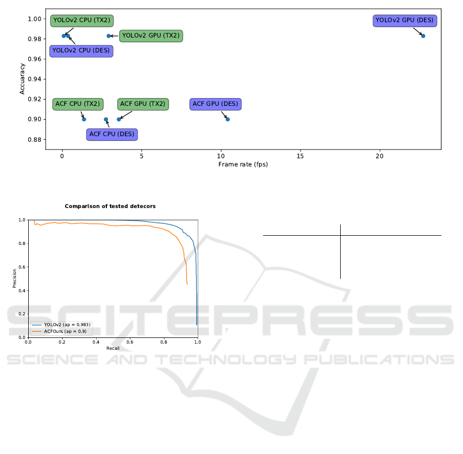
Figure 5: Comparison of the tested detectors in both speed and accuracy.

Figure 4: Comparison between tested detectors, “ACFOurs”

represents our ACF implementations, “YOLOv2” is the

standard YOLOv2 object detector.

is a criteria that is at least as important. In table 4

we compare the tested detectors in terms of running

speed. Because the main purpose of our ACF imple-

mentation was to use it in conjunction with some sort

of scene constraints, which only require evaluation of

one scale, we only have an implementation to evalu-

ate one scale. The results in the table are estimations

based on the speedups we got in section 5. As be-

fore the speed of the different detectors are tested on

the 1920x1080 TownCenter dataset. In terms of speed

the GPU ACF port still appears to perform better on

TX2 compared to YOLOv2 (281 ms vs 343 ms). On

the desktop GPU however, this is not the case. YO-

LOv2 is more than twice as fast as the ACF GPU port.

If there is no GPU available on the system the clear

winner is ACF. ACF is still capable of running quite

fast on CPU alone, YOLOv2 is much slower making

it unusable on CPU for time sensitive applications.

Figure 5 visualises the speed / accuracy trade-off.

Table 4: Comparison of total processing times of the tested

detectors on both CPU and GPU.

DES (ms) TX2 (ms)

ACF (CPU) 364 731

ACF (GPU) 96 281

YOLOv2 (CPU) 2805 11289

YOLOv2 (GPU) 44 343

7 CONCLUSION

In this paper we described how a pre-deep lear-

ning detector which uses handcrafted features such as

ACF, can be sped up by utilizing the GPU. We evalu-

ated our GPU implementation on two platforms, the

embedded Jetson TX2 GPU platform, and a desktop

equipped with a NVIDIA GTX 1080. While the ACF

detector does not lend itself easily to big speedups by

parallelizing (especially the evaluation step) we still

managed to get some signiﬁcant speed increases on

both tested platforms. Compared to the state-of-the-

art deep learning detector YOLOv2 we still manage

to get the fastest detections using the GPU ACF met-

hod on a TX2. YOLOv2 is however more accurate, as

could be expected taking into account the fast (deep

learning based) evolution object detection techniques

have seen in recent years. It is likely that in the fu-

ture deep learning methods, will overtake traditional

methods in the ﬁeld of real time embedded systems as

they have with much of the rest of the ﬁeld of object

detection. As for right now, we would say that tra-

ditional methods still have their place on embedded

platforms.

The tested deep learning methods do also require

the presence of a powerful GPU, if no GPU is pre-

sent, as is the case with many low-power embedded

platforms (the TX2 is an exception in this case), tra-

GPU Accelerated ACF Detector

247

ditional methods still win by a wide margin in terms

of speed.

ACKNOWLEDGMENTS

This work is supported by the agency Flanders In-

novation & Entrepreneurship (VLAIO) and the com-

pany Robovision.

REFERENCES

Bell, N. and Hoberock, J. (2011). Thrust: A productivity-

oriented library for cuda. GPU computing gems Jade

edition, 2:359–371.

Benfold, B. and Reid, I. (2011). Stable multi-target tracking

in real-time surveillance video. In CVPR, pages 3457–

3464.

Dalal, N. and Triggs, B. (2005). Histograms of oriented gra-

dients for human detection. In Computer Vision and

Pattern Recognition, 2005. CVPR 2005. IEEE Com-

puter Society Conference on, volume 1, pages 886–

893. IEEE.

Doll

ar, P., Appel, R., Belongie, S., and Perona, P. (2014).

Fast feature pyramids for object detection. IEEE

Transactions on Pattern Analysis and Machine Intel-

ligence, 36(8):1532–1545.

Doll

ar, P., Tu, Z., Perona, P., and Belongie, S. (2009). Inte-

gral channel features.

Felzenszwalb, P., McAllester, D., and Ramanan, D. (2008).

A discriminatively trained, multiscale, deformable

part model. In Computer Vision and Pattern Recog-

nition, 2008. CVPR 2008. IEEE Conference on, pages

1–8. IEEE.

Freund, Y. and Schapire, R. E. (1995). A desicion-theoretic

generalization of on-line learning and an application

to boosting. In European conference on computatio-

nal learning theory, pages 23–37. Springer.

Jones, S. (2012). Introduction to dynamic parallelism. In

GPU Technology Conference Presentation S, volume

338, page 2012.

Lin, T.-Y., Maire, M., Belongie, S., Hays, J., Perona, P.,

Ramanan, D., Doll

ar, P., and Zitnick, C. L. (2014).

Microsoft coco: Common objects in context. In Euro-

pean conference on computer vision, pages 740–755.

Springer.

Liu, W., Anguelov, D., Erhan, D., Szegedy, C., Reed, S., Fu,

C.-Y., and Berg, A. C. (2016). Ssd: Single shot mul-

tibox detector. In European conference on computer

vision, pages 21–37. Springer.

Obukhov, A. (2011). Haar classiﬁers for object detection

with cuda. GPU Computing Gems Emerald Edition,

pages 517–544.

Pedersoli, M., Vedaldi, A., Gonzalez, J., and Roca, X.

(2015). A coarse-to-ﬁne approach for fast deformable

object detection. Pattern Recognition, 48(5):1844–

1853.

Redmon, J. and Farhadi, A. (2016). Yolo9000: Better, fas-

ter, stronger. arXiv preprint arXiv:1612.08242.

Tijtgat, N., Ranst, W. V., Volckaert, B., Goedem

e, T., and

Turck, F. D. (2017). Embedded real-time object de-

tection for a UAV warning system. 1st International

Workshop on Computer Vision for UAVs.

Van Beeck, K. (2016). The automatic blind spot camera:

hard real-time detection of moving objects from a mo-

ving camera.

Viola, P., Jones, M. J., and Snow, D. (2003). Detecting

pedestrians using patterns of motion and appearance.

In null, page 734. IEEE.

VISAPP 2018 - International Conference on Computer Vision Theory and Applications

248